A Suggestion for Clear Pandas Implementation

30 Jun 2025 in Blog

Pandas implementation practices that advocates for transformation-centric design inducing high code readability and modularization.

Code: Github

Pandas Get Dirty Sometimes

panda is a powerful tool for working with tabular data, offering a wide range of built-in functions that make data transformation tasks straightforward. However, I’ve noticed that as more tables are integrated and transformations accumulate, the code tends to get “dirty” fast: the logic becomes harder to follow, and it’s easy to overlook certain steps—especially when reusing the same transformation chains across similar tables.

It’s natural to wrap these transformations into functions to make them more manageable. But I don’t think that’s the best long-term solution.

Ideally, I want to establish a systematic way of organizing the code before I even begin, so that the logic is structured, maintainable, and easy to read from the outset. That’s the purpose of this blog.

In the sections that follow, I’ll outline how I translate data-related entity concepts into code, along with a brief guide on assembling them into a working pipeline.

• The Concept
• The Implementation
  • DataConnector
  • Transform
• The Assemble
• Summary

The Concept

To me, a data pipeline is simple: it’s a graph whose nodes are either DataConnector or transform. A DataConnector handles reading from and writing to data sources, regardless of their origin. A transform handles the self-transform or multi-table interaction logic, for example an outer join. These two entities communicate by accepting and returning pandas.DataFrame objects. Together, they provide everything you need to build a functional Pipeline.

As more tables come into play, these entities need to be organized into groups. Each group should have a clear, descriptive name that reflects the transformation objective it performs. As a starting point, I typically use the classic ETL (Extract, Transform, Load) structure to guide the grouping. If the logic becomes more complex, I introduce intermediate groups to maintain clarity and modularity.

Fig. 1 summarizes the core concepts, their semantic interactions, and how they are grouped.

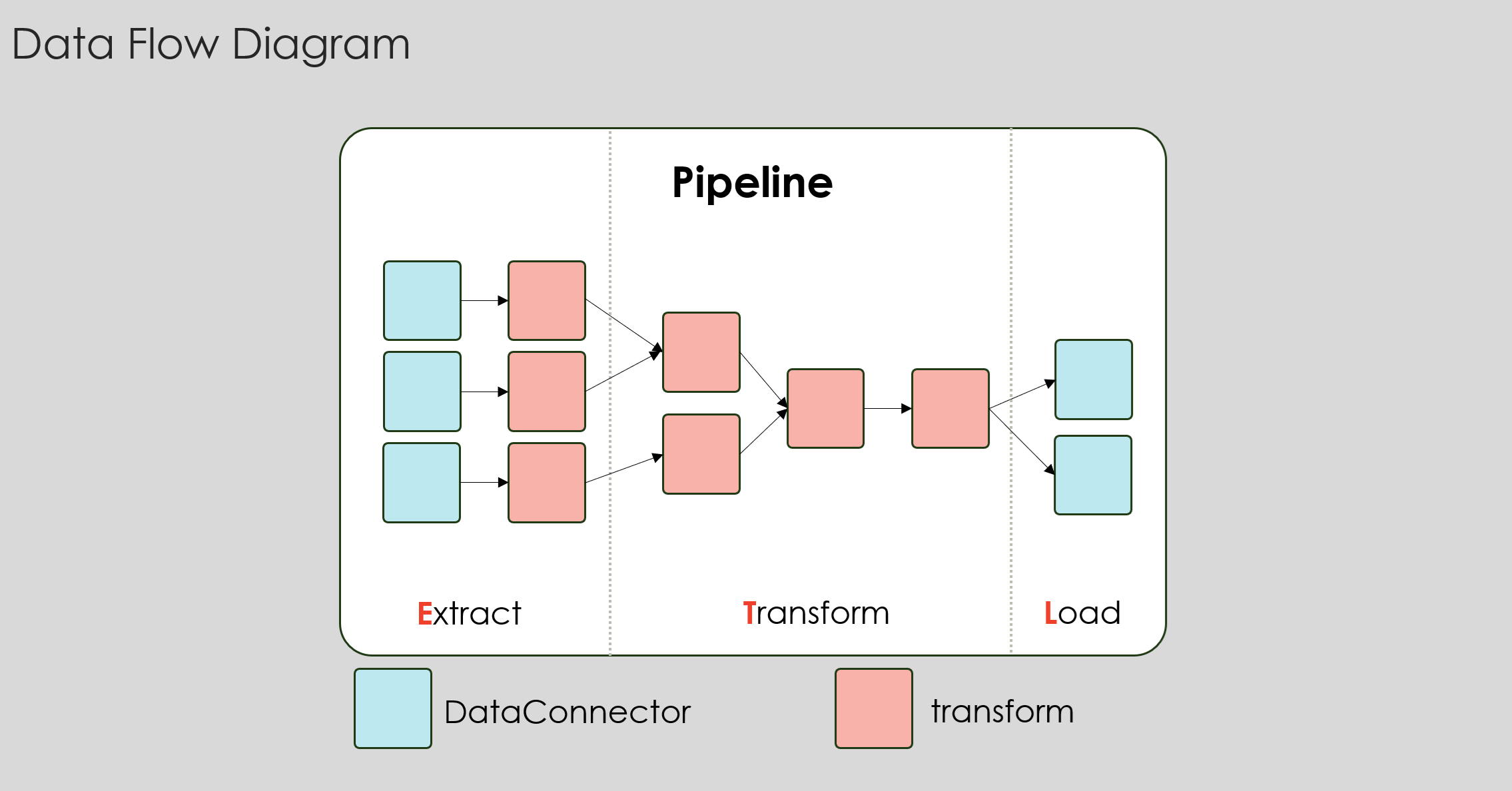Fig. 1. The concept of entities in a data pipeline.

The Implementation

DataConnector

Developers can delegate and abstract away the task of establishing connections and querying from various data sources through a unified interface, namely DataConnector.

class DataConnector:
    def __init__(self, source):
        self.source = source

    def get_data(self, query: str = None) -> pd.DataFrame:
        pass
    
    def write_data(self, pd_table: pd.DataFrame):
        pass

All concrete connectors adhere to this interface and implement their source-specific logic by inheriting from DataConnector. While this example assumes a pure Python workflow, the same structure can be adapted for PySpark by replacing all instances of pandas.DataFrame with pyspark.sql.DataFrame. Notably, the duckdb package enables SQL-query support as long as the loaded table is stored in a variable named df. This eliminates the need to come up with a meaningful table names in small utility functions—a convenience I strongly recommend applying later in transform as well.

class CSVConnector(DataConnector):
    def __init__(self, source):
        self.source = source

    def get_data(self, query: str = None)-> pd.DataFrame:
        df = pd.read_csv(self.source)
        if (query):
            con = duckdb.connect()
            df = con.execute(query).df()
        return df
    
    def write_data(self, df: pd.DataFrame):
        df.to_csv(self.source, index=False)

We can take the abstraction one step further by removing the need for developers to manually select the appropriate connector. Instead, we delegate that responsibility to a ConnectorFactory:

class ConnectorFactory:
    @staticmethod
    def create_connector(source: str) -> DataConnector:
        if source.endswith('.csv'):
            return CSVConnector(source)
        elif source.endswith('.xlsx'):
            return ExcelConnector(source)
        else:
            raise ValueError("Unsupported file format. Use .csv or .xlsx") 

With this setup, input/output operations can be cleanly abstracted using get_data() and write_data(), even as concise one-liners if desired:

customer_connector = ConnectorFactory().create_connector('data/customers.csv')
customer_table = customer_connector.get_data("SELECT * FROM df WHERE c_acctbal > 200")

order_details_connector = ConnectorFactory().create_connector('data/urgent_order_details.csv')
order_details_connector.write_data(data['urgent_order_details']) 

Transform

One of the strengths of pandas is how naturally pipe supports chaining transformations in the order they’re applied—making the logic both intuitive and readable. Each transformation operates on a complete pandas.DataFrame and returns a new one, which eliminates the ambiguity that can arise from using an inplace argument. You can safely name your working variable df without overthinking it — unless multiple dataframes are involved. Another benefit is testability: each transformation function can be developed and verified independently. Once it works, you can drop it into the chain like a perfectly shaped LEGO piece.

transform.customers.py

def round_up_acctbal(df: pd.DataFrame) -> pd.DataFrame:
    # Function to round up 'c_acctbal' values to the nearest integer
    def round_value(value):
        if pd.isna(value):
            return value
        return round(value, 2) if value >= 0 else round(value, 0)
    
    df['c_acctbal'] = df['c_acctbal'].apply(round_value)
    return df

def filter_customers(df: pd.DataFrame, max_custkey: int) -> pd.DataFrame:
    return df[df['c_custkey'] <= max_custkey]

main.py

from src import transform
processed_customer_table = (
            customer_table
            .pipe(transform.customers.round_up_acctbal)
            .pipe(transform.customers.filter_customers, max_custkey=1000)
            )

The chaining syntax also implies that each transformation is applied to derive a specific table. This allows you to name your functions using a clear verb + object convention, without needing to repeat the table name in the function itself. To keep things organized, you can group related transformation functions by their target table - e.g., customers.py, orders.py - and place shared utilities in a common base.py module:

📦 my_project 
├── 📁 src
|    ├── 📁 transform 
│    |   ├── 📄 base.py 
│    |   ├── 📄 customers.py 
│    |   └── 📄 orders.py 
...

Lastly, by fully embracing the use of pipe, each table name ideally appears in just two places: where it’s created, and where it’s used as input to compute a downstream table. This mirrors the concept of data lineage, as it makes it easier to trace how a table is produced and understand its downstream dependencies.

The Assemble

At this point, you have all the essential ingredients to build a data pipeline. For simple use cases, the pipeline can be implemented directly in the entry point, such as main.py. For more complex scenarios, it’s helpful to define a Pipeline class that clearly groups transformations — leaving placeholders to be filled with the appropriate functions. To give you a complete picture, here’s how all the entities relate to one another:

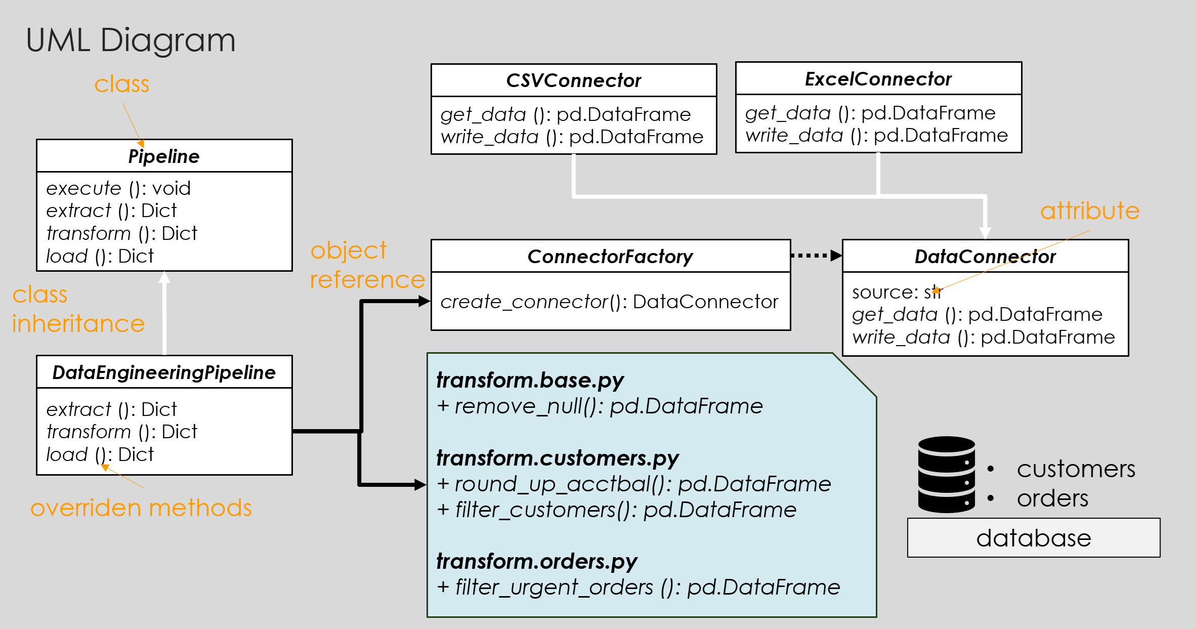Fig. 2. Diagram illustrated relationship between OOP implementation of pipeline entities.

As I applied this framework to my own project, I encountered a few variations and adapted accordingly:

• I grouped transformations into three categories:
  • Source: data retrieval and extraction
  • Transformation: filtering, joining, deriving, aggregating
  • Output: storing, visualizing, or exporting results
• Some tables are loaded once and serve only to enrich other tables with additional columns. For these, I chose to load and apply them within a single function tied to the main table. This makes it easier to trace where these auxiliary tables are used.
• In machine learning projects, I typically treat model scoring as part of the Transformation phase.
• When a joined table serves a new analytical purpose—beyond simple enrichment—I treat it as a new table altogether. From a transformation perspective, both pd.merge() and pipe() are valid expression in this case.

Summary

This pipeline-design guideline is structured around four core entities that work together to manage data flow and transformation:

• Connector: Responsible for reading data from and writing data to external sources. It acts as the interface between the pipeline and the outside world (e.g., databases, files, APIs).
• Transform: Handles intermediate data processing. Each transform takes in data, applies a specific transformation logic, and outputs the modified data for the next step.
• Dataframe: Serves as the data container passed between connectors and transforms. It represents the input and output at each stage of the pipeline, ensuring consistency and traceability of the data.
• Pipeline: Orchestrates the sequence of connectors and transforms. It defines the overall workflow by chaining these components into a cohesive process, enabling modular and reusable data operations.

This design promotes clarity, modularity, and flexibility, making it easy to build, maintain, and extend data workflows.

You can check out a runnable example pipeline at my Github repo 👉 clearpandas.

---