Event Study: A Framework From Economics That Every Data Scientist Should Know
in Blog
There is a method in empirical economics that has been quietly doing what data scientists now call causal inference since the 1930s. It is called the event study. The canonical reference is A. Craig MacKinlay’s 1997 paper in the Journal of Economic Literature, and while the paper frames everything around stock prices and earnings announcements, the underlying machinery is general enough to apply to almost any time series problem where you want to measure the effect of a well-defined event.
This post is a walkthrough of that machinery — the intuition, the mathematics, and a deliberate translation into modern DS language at each step. I came to this through a careful reading of the MacKinlay paper, and the translation exercise turned out to be genuinely illuminating. If you work in operations, platform engineering, product analytics, or applied ML, there is probably a problem in your backlog that this framework fits better than whatever you are currently reaching for.
- The Core Idea
- The Fundamental Formula
- Normal Return Models
- The Timeline Architecture
- Statistical Assumptions and What They Actually Mean
- Estimation: OLS on the Market Model
- Statistical Tests
- On Returns vs. Raw Values
- Applications Beyond Finance
- Python Packages
- Summary
The Core Idea
The goal of an event study is to measure the effect of a well-defined economic event on the value of a firm. MacKinlay’s starting observation is elegant: if markets are rational, the impact of an event will be reflected immediately in security prices. You do not need to model the entire economy to measure this impact — you just look at the price reaction.
More precisely, the method asks: what would the stock price have done had the event not occurred? That counterfactual is called the normal return. The difference between what actually happened and what the model says should have happened is the abnormal return — the event’s fingerprint in the data.
This framing should already feel familiar. In modern data science terms:
An event study measures whether the residuals from a baseline model behave non-randomly around a specific point in time.
The entire apparatus — estimation windows, market models, cumulative abnormal returns — is an elaboration of that one sentence.
The Fundamental Formula
MacKinlay’s first formula is: \[AR_{it} = R_{it} - E(R_{it} | X_t)\]
where \(AR_{it}\) is the abnormal return for firm \(i\) on day \(t\), \(R_{it}\) is the actual return, and \(E(R_{it} \| X_t)\) is the normal return given conditioning information \(X_t\).
Before going further, we need to clarify what a return is. In finance, the return \(R_{it}\) is the percentage change in the stock price from one day to the next: \[R_{it} = \frac{P_{it} - P_{i,t-1}}{P_{i,t-1}}\]
where \(P_{it}\) is the price of firm \(i\) on day \(t\). In practice, researchers often prefer the log return: \[R_{it} = \ln\left(\frac{P_{it}}{P_{i,t-1}}\right)\]
Log returns are preferred because they are additive over time (a nice mathematical property) and more likely to be normally distributed. For small daily price changes the two are nearly identical.
Using percentage changes rather than raw prices matters because raw prices are non-stationary — they drift and trend over time, which breaks the regression assumptions the method relies on. Returns fluctuate around a stable mean, which is what we need. We return to this point later when discussing whether the framework applies to raw values in non-finance settings.
Now, the \(E(\cdot)\) notation in MacKinlay’s formula looks like a probabilistic expectation, and it is — but a specific kind. It is not a forecast about the future. It is the model’s predicted value of what firm \(i\) should return on day \(t\), given what we know, if no event had occurred. In modern DS notation: \[AR_{it} = R_{it} - \hat{R}_{it}\]
where \(\hat{R}_{it}\) is the fitted value from your baseline model. The full mapping:
| MacKinlay | Modern DS |
|---|---|
| \(R_{it}\) | \(y\) (actual outcome) |
| \(E(R_{it} | X_t)\) | \(\hat{y}\) (model prediction) |
| \(AR_{it}\) | residual \(= y - \hat{y}\) |
| \(X_t\) | features / conditioning information |
MacKinlay writes \(E(\cdot)\) rather than \(\hat{y}\) because he wants to stay agnostic about which model generates the prediction. Depending on your choice of baseline model, \(X_t\) changes: it might be nothing (constant mean model), the market return (market model), or a set of risk factors (APT model). The notation unifies all cases behind a single symbol.
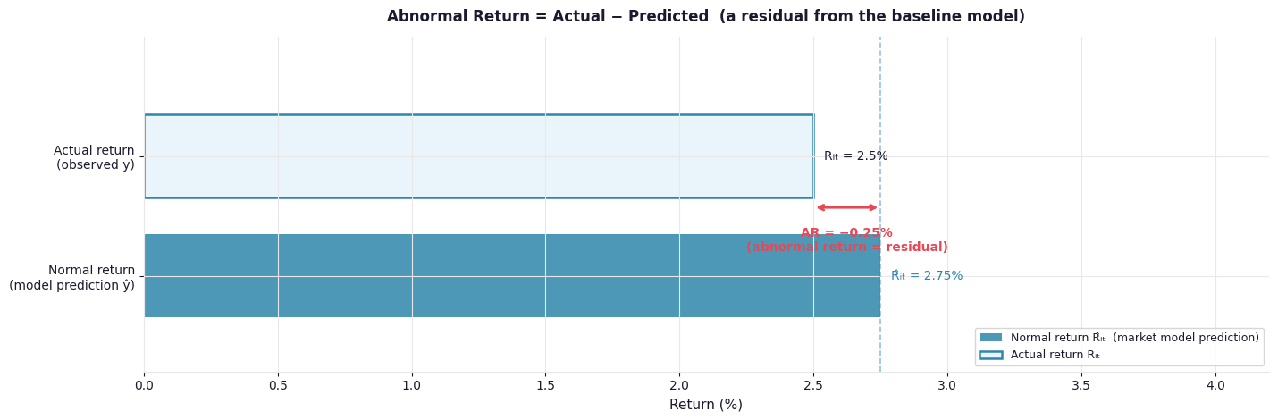 Fig. 1. The abnormal return is the gap between what a firm actually returned and what the baseline model predicted. In DS terms, it is an out-of-sample residual.
Normal Return Models
The baseline model — what MacKinlay calls the normal return model — determines the quality of the counterfactual. Two models are central to the paper.
The Constant Mean Return Model
\[R_{it} = \mu_i + \varepsilon_{it}\]This is the simplest possible baseline. The normal return for firm \(i\) on any day is just its historical average return \(\mu_i\), estimated as the sample mean over a pre-event window. The abnormal return is then: \[AR_{it} = R_{it} - \hat{\mu}_i\]
In regression terms, this is a model with an intercept and no features. It is fast to estimate and easy to understand, but it has a fundamental weakness: it cannot distinguish market-wide movements from firm-specific effects.
Consider what happens on an event day when the whole market rises 3% and the firm’s stock also rises 2.5%. The constant mean model sees a large positive abnormal return. But the stock may have risen simply because the whole market did. The event may have had no effect — or even a slightly negative one. The model has no way to tell.
The Market Model
\[R_{it} = \alpha_i + \beta_i \cdot R_{mt} + \varepsilon_{it}\]where \(R_{mt}\) is the return of the market portfolio on day \(t\) — in practice, an index like the S&P 500 or the CRSP value-weighted index. \(\beta_i\) captures how sensitive firm \(i\) is to market-wide movements. \(\alpha_i\) captures the firm’s average return net of market exposure.
The abnormal return becomes: \[AR_{it} = R_{it} - \hat{\alpha}_i - \hat{\beta}_i \cdot R_{mt}\]
To make \(\hat{\alpha}_i\) and \(\hat{\beta}_i\) concrete: \(\hat{\beta}_i\) is the stock’s sensitivity to the market, estimated from historical data. A stock with \(\hat{\beta}_i = 0.9\) has historically moved 0.9% for every 1% the market moves. \(\hat{\alpha}_i\) is the stock’s average daily return after removing the market’s contribution — for most stocks this is a small number close to zero, typically around 0.03–0.05% per day.
Return to the same example: market rises 3%, stock rises 2.5%, \(\hat{\beta}_i = 0.9\), and \(\hat{\alpha}_i = 0.05\%\). The model predicts \(0.05\% + 0.9 \times 3\% = 2.75\%\). The abnormal return is \(2.5\% - 2.75\% = -0.25\%\). The event was actually slightly negative once the market-wide movement is stripped out.
One important clarification on \(R_{mt}\): because a single firm has negligible weight in a broad market index, \(R_{mt}\) is treated as exogenous — an observed external input, not a model prediction. In regression terms: \(R_{it}\) is your target (\(y\)), \(R_{mt}\) is your feature (\(X\)). Knowing \(R_{mt}\) does not tell you \(R_{it}\) exactly; it only explains the fraction of \(R_{it}\) that moves with the market. The residual is what the market cannot explain, and that is where the signal lives.
This is why the market model dominates in practice. It removes a known, measurable source of variance before you measure the thing you care about. Lower residual variance means sharper hypothesis tests.
 Fig. 2. The constant mean model conflates market-wide movement with firm-specific effects. The market model strips the common factor first, leaving a cleaner signal. Note the smaller residual (AR) in the right panel on the event day.
The Timeline Architecture
The event study has a precise temporal structure with three distinct windows.
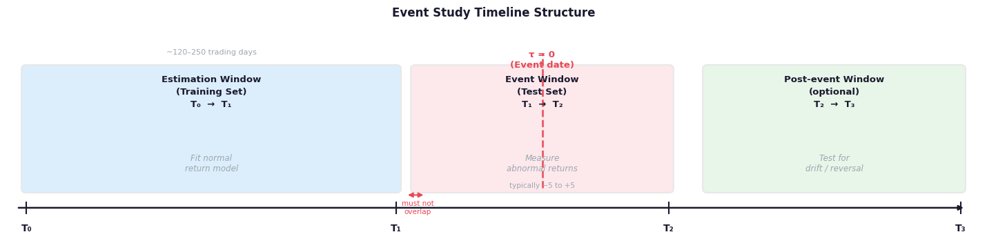 Fig. 3. The three-window structure of an event study. The estimation and event windows must not overlap — otherwise the event contaminates the baseline model.
Estimation window (\(T_0\) to \(T_1\)): The period used to fit the normal return model. Typically 120 to 250 trading days before the event. Parameters are estimated here and then frozen.
Event window (\(T_1\) to \(T_2\)): The period where abnormal returns are measured. Centered on day \(\tau = 0\) (the event date). Typically \(-1\) to \(+1\) or \(-5\) to \(+5\) days, depending on how precisely the event date is known and how quickly the market is expected to react.
Post-event window (optional): Used to test for drift or reversal after the initial reaction.
The critical design rule: estimation and event windows must not overlap. If the event contaminates the baseline model estimation, your counterfactual is invalid. This maps directly to the DS principle of not using test data during training.
Statistical Assumptions and What They Actually Mean
MacKinlay imposes that asset returns are jointly multivariate normal and independently and identically distributed (IID) through time. This is doing three distinct things simultaneously, and each carries real implications.
Joint Multivariate Normality
All asset returns at time \(t\) follow a multivariate normal distribution: \(\mathbf{R}_t \sim \mathcal{N}(\boldsymbol{\mu}, \boldsymbol{\Sigma})\). The practical consequence is that the conditional mean \(E(R_{it} \| R_{mt})\) is linear in \(R_{mt}\) — a direct property of the multivariate normal. This is what makes the market model correctly specified: joint normality guarantees that the linear regression is the right functional form, not just an approximation.
Independence Through Time
\(R_t \perp R_s\) for all \(t \neq s\). No autocorrelation; today’s return carries no predictive information about tomorrow’s. This is the weak form of market efficiency baked into the statistical assumption. Without it, OLS standard errors would be wrong and the hypothesis tests unreliable.
Identical Distribution Through Time
The same parameters govern every time period. \(\alpha_i\) and \(\beta_i\) are stationary — they do not drift between the estimation window and the event window. This is what makes the counterfactual credible: the model trained on pre-event data describes what would have happened during the event window, had the event not occurred.
In practice: all three are approximate. Returns have fat tails, volatility clustering, and drifting betas. The framework is reasonably robust to moderate violations, especially when aggregated across many events (the Central Limit Theorem normalizes the aggregate even when individual returns are non-normal). Long-horizon studies are more vulnerable, which is why they have a separate and messier literature.
Estimation: OLS on the Market Model
Given the IID and normality assumptions, OLS is the appropriate estimator. The intuition behind OLS is simple: find the parameter values \(\hat{\alpha}_i\) and \(\hat{\beta}_i\) that minimize the sum of squared prediction errors over the estimation window: \[\min_{\alpha, \beta} \sum_{t=T_0+1}^{T_1} \left( R_{it} - \alpha_i - \beta_i \cdot R_{mt} \right)^2\]
Geometrically, this finds the line through the cloud of \((R_{mt}, R_{it})\) points that sits as close as possible to all of them simultaneously. The residuals — vertical distances from each point to the fitted line — are exactly what become abnormal returns in the event window.
In matrix form, stacking \(L\) observations from the estimation window:
- \(\mathbf{y}\): \(L \times 1\) vector of firm returns \([R_{i,T_0+1}, \ldots, R_{i,T_1}]^\top\)
- \(\mathbf{X}\): \(L \times 2\) design matrix with a column of ones and a column of market returns
- \(\boldsymbol{\theta}_i = [\alpha_i, \beta_i]^\top\): parameter vector
The OLS solution is: \[\hat{\boldsymbol{\theta}}_i = (\mathbf{X}^\top \mathbf{X})^{-1} \mathbf{X}^\top \mathbf{y}\]
In scalar form: \[\hat{\beta}_i = \frac{\text{Cov}(R_{it}, R_{mt})}{\text{Var}(R_{mt})}, \qquad \hat{\alpha}_i = \hat{\mu}_i - \hat{\beta}_i \cdot \hat{\mu}_m\]
The residual variance is estimated as: \[\hat{\sigma}^2_{\varepsilon_i} = \frac{1}{L-2} \sum_{t} \hat{\varepsilon}^2_{it}\]
divided by \(L - 2\) because two degrees of freedom were consumed estimating \(\alpha_i\) and \(\beta_i\).
Once estimated, parameters are frozen. On event day \(\tau\), the out-of-sample abnormal return is: \[AR_{i\tau} = R_{i\tau} - \hat{\alpha}_i - \hat{\beta}_i \cdot R_{m\tau}\]
This is a genuine out-of-sample prediction error. The model never saw the event window data. That separation is what gives the abnormal return its causal interpretation.
Statistical Tests
To understand the need for statistical testing, consider a concrete stock market example. Suppose a pharmaceutical company announces clinical trial results on day \(\tau = 0\). Its stock rises 4% that day. Is this unusual? Maybe the whole biotech sector rose 3.8% that day, and this firm’s \(\hat{\beta}_i = 1.05\), making the predicted return \(3.99\%\). The abnormal return would be just \(+0.01\%\) — essentially nothing. Alternatively, if the market was flat and the firm still rose 4%, that would be genuinely surprising. The statistical test formalizes this intuition: it asks how likely such an abnormal return would be under the null hypothesis that no event effect exists.
The Variance of a Single Abnormal Return
\(AR_{i\tau}\) carries uncertainty from two sources. Even with perfect parameters, there would be genuine day-to-day randomness \(\sigma^2_{\varepsilon_i}\). On top of that, the estimated parameters \(\hat{\alpha}_i\) and \(\hat{\beta}_i\) carry sampling error from a finite estimation window. MacKinlay shows: \[\text{Var}(AR_{i\tau}) = \sigma^2_{\varepsilon_i} \left[ 1 + \frac{1}{L} + \frac{(R_{m\tau} - \hat{\mu}_m)^2}{L \cdot \hat{\sigma}^2_m} \right]\]
| Term | What it captures |
|---|---|
| \(\sigma^2_{\varepsilon_i} \cdot 1\) | Irreducible daily noise |
| \(\sigma^2_{\varepsilon_i} / L\) | Estimation error in \(\hat{\alpha}_i\) |
| \(\sigma^2_{\varepsilon_i} \cdot (R_{m\tau} - \hat{\mu}_m)^2 / (L \cdot \hat{\sigma}^2_m)\) | Estimation error in \(\hat{\beta}_i\), amplified when the event-day market return is unusual |
The third term is a leverage effect familiar from OLS: if the event day has an unusual market return, you are extrapolating \(\hat{\beta}_i\) into unfamiliar territory, adding variance. For large \(L\), both correction terms vanish and \(\text{Var}(AR_{i\tau}) \approx \sigma^2_{\varepsilon_i}\).
Single Day, Single Firm
The standardized abnormal return: \[SAR_{i\tau} = \frac{AR_{i\tau}}{\hat{\sigma}_{\varepsilon_i}} \sim t(L-2)\]
Because \(\hat{\sigma}_{\varepsilon_i}\) is estimated rather than known, the distribution is a \(t\) with \(L - 2\) degrees of freedom. For \(L = 250\), this is indistinguishable from \(\mathcal{N}(0, 1)\) in practice.
Reject \(H_0\) (no event effect) if \(\|SAR_{i\tau}\| > 1.96\) at the 5% significance level.
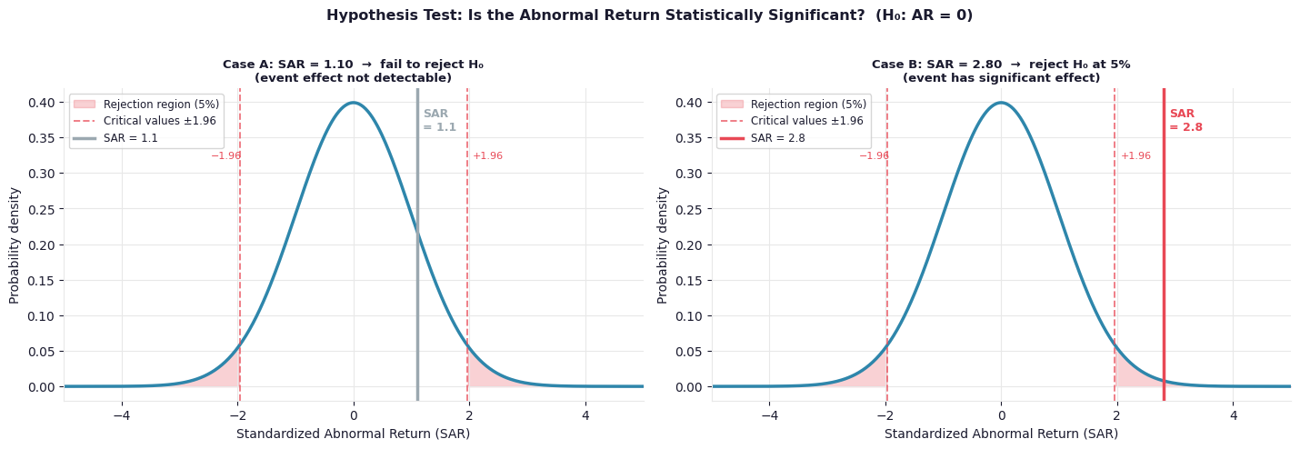 Fig. 4. Two single-firm cases under the same N(0,1) null distribution. In Case A, the standardized abnormal return of 1.10 falls within the non-rejection region — the event effect is not detectable above the noise. In Case B, an SAR of 2.80 falls well into the rejection region — strong evidence the event had a real effect.
Aggregating Across Time: CAR
For a single firm over an event window of \(T\) days: \[CAR_i(\tau_1, \tau_2) = \sum_{\tau=\tau_1}^{\tau_2} AR_{i\tau}\] \[\text{Var}(CAR_i) = T \cdot \sigma^2_{\varepsilon_i}\] \[Z_i = \frac{CAR_i}{\sqrt{T \cdot \hat{\sigma}^2_{\varepsilon_i}}} \sim \mathcal{N}(0, 1)\]
Note that variance grows linearly with window length. A wider event window captures more of the effect if it is gradual, but also accumulates more noise. The signal-to-noise ratio improves with window width only if the true effect genuinely persists across multiple days.
Aggregating Across Firms: CAAR
The real statistical power of the method comes from averaging across \(N\) firms experiencing the same type of event: \[CAAR(\tau_1, \tau_2) = \frac{1}{N} \sum_i CAR_i\] \[\text{Var}(CAAR) = \frac{\sigma^2}{N} \quad \text{(assuming cross-sectional independence)}\] \[Z = \frac{CAAR}{\sqrt{\text{Var}(CAAR)}} \sim \mathcal{N}(0, 1)\]
Variance shrinks at rate \(1/N\). This is the Central Limit Theorem at work: idiosyncratic noise averages out across firms while the true event effect, if it exists, persists in the mean. The cross-sectional independence assumption — that \(CAR_i\) and \(CAR_j\) are uncorrelated across firms — is what makes this reduction valid. It holds when events are spread across calendar time. When events cluster on the same date (e.g. all firms react to the same macro announcement), the correlations stack rather than average out, and the test statistic is inflated — a separate complication MacKinlay addresses in the clustering section.
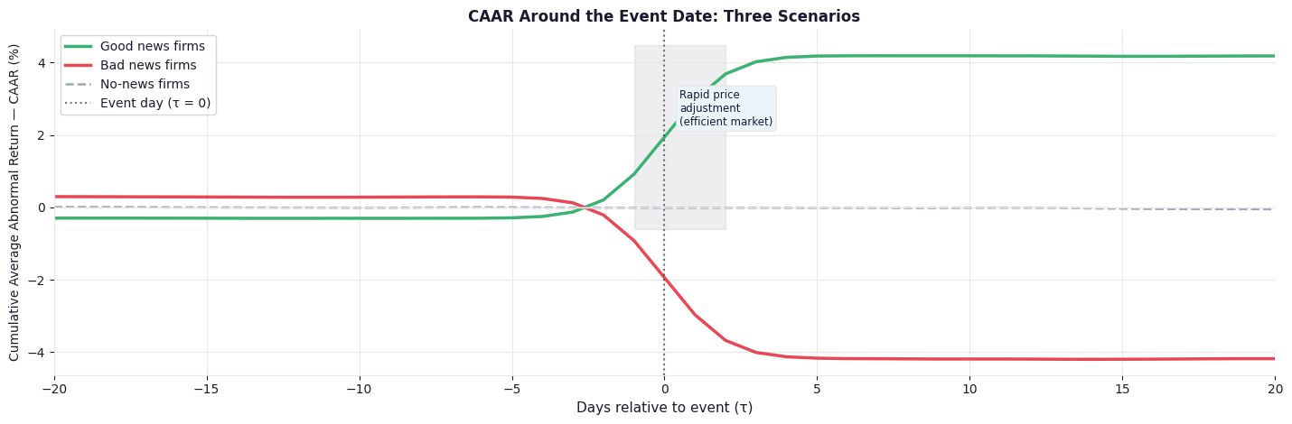 Fig. 5. The characteristic CAAR plot around an event date. A sharp jump at \(\tau = 0\) is consistent with market efficiency — information gets priced in immediately. A gradual post-event drift would suggest delayed price discovery. A flat line means the event carried no new information for the market.
On Returns vs. Raw Values
MacKinlay uses returns (percentage changes) rather than raw prices for three reasons.
Stationarity. Raw prices trend and drift — they are non-stationary. Returns fluctuate around a stable mean, making the IID assumption at least approximately defensible. OLS on non-stationary data produces spurious regressions: high \(R^2\), significant-looking coefficients, but entirely meaningless results driven by shared trends rather than genuine relationships.
Comparability. A $1 move means completely different things for a $5 stock and a $500 stock. Returns normalize everything to a common percentage scale, making cross-firm aggregation meaningful.
Multiplicative process. Stock prices compound multiplicatively. Log returns are additive over time, which matches how the underlying price process actually works.
For non-finance applications, the question is whether your raw metric has these same properties. The answer depends on the specific series, not the framework:
- If your metric already fluctuates around a stable mean (CPU utilization, daily fault count, vessel turnaround time in hours), it is already behaving like a return. Use raw values directly.
- If your metric has a trend or drift (cumulative throughput, a growing user base), difference it first: \(\Delta y_t = y_t - y_{t-1}\).
- If your metric has seasonality, remove the seasonal component before applying the framework.
The practical check is simple: fit your baseline model on the estimation window and plot the residuals. If they look like white noise around zero, your transformation is sufficient. If they show drift or cycles, you are not done yet.
The event study machinery is agnostic to transformation. What it requires is that the residuals going into the hypothesis test are well-behaved.
Applications Beyond Finance
The framework generalizes to any domain with a time series outcome, a well-defined event date, and a credible normal behavior model. The literature has extended it widely.
Information systems and cybersecurity. Researchers measure the stock market cost of data breach disclosures using the abnormal return framework, with the breach announcement date as the event. The same logic applies in reverse: use pre-incident operational metrics as the baseline, and measure whether system behavior deviates abnormally around known incident dates.
Marketing. New product launches, CMO appointments, brand acquisitions — all have been studied as events with stock price impact as the outcome. The framework applies equally to non-financial outcomes: does customer sentiment score show an abnormal shift around a campaign launch date?
Operations and supply chain. Disruptions, recalls, and contract announcements have measurable effects on throughput and lead time metrics. The event study provides a rigorous way to separate the disruption’s effect from background variability.
Policy evaluation. This is the most important generalization. Event studies are structurally equivalent to a generalization of Difference-in-Differences. In a staggered treatment setting — where different units receive a policy change at different times — units treated later serve as the control for units treated earlier. No “never treated” group is required. Every feature launch evaluation, every policy change measured on panel data, is operating in event study territory.
NLP and social media. Earnings announcements have been used as events with Twitter sentiment as the outcome variable — measuring whether public sentiment shows abnormal shifts around corporate disclosures, and in which direction.
The unifying structure across all of these is:
| MacKinlay Concept | General DS Translation |
|---|---|
| Security return \(R_{it}\) | Any measurable time series metric |
| Market return \(R_{mt}\) | Baseline control signal (trend, peer average, seasonal pattern) |
| Normal return model | Regression trained on pre-event data |
| Estimation window | Training set |
| Event window | Test set |
| Abnormal return | Out-of-sample residual |
| \(CAR\) | Cumulative residual over event window |
| \(CAAR\) | Average cumulative residual across many events |
| \(H_0: CAAR = 0\) | Event had no systematic effect on the metric |
Python Packages
Several mature Python packages implement the event study workflow, saving you from building the estimation and testing machinery from scratch.
eventstudy is the most direct implementation of the MacKinlay framework. It supports the constant mean and market model, handles the estimation and event window split, and computes ARs, CARs, and significance tests out of the box. A good starting point if you are applying the method to financial return data.
statsmodels does not have a dedicated event study module, but its OLS and time series tools give you everything you need to build the framework manually. This is often the right choice when your normal return model is more complex than the market model, or when you want full control over the test statistic construction.
For the figures and simulation work in this post, standard numpy and matplotlib were sufficient — the core computations are straightforward once the framework is understood.
Summary
The event study is a complete, self-consistent framework for measuring the effect of an intervention on a time series metric. Its three contributions, each worth keeping distinct:
The causal logic. The counterfactual is explicit: what would the metric have been without the event? The baseline model formalizes that counterfactual, and the abnormal value is the difference between reality and the model’s prediction. This is more rigorous than naive before/after comparisons, which conflate the event’s effect with ongoing trends and external shocks.
The statistical machinery. Abnormal returns are residuals with known distributional properties under the model assumptions. Aggregating across time gives CAR; aggregating across events gives CAAR. The variance structure is tractable — it shrinks at rate \(1/N\) across events, giving real statistical power when you have many observations of the same event type. The test statistics are standard normal under the null.
The generalizability. The framework requires a stationary outcome metric, a well-defined event date, a credible baseline model, and approximately IID residuals under the null. Stock prices happen to satisfy these naturally; other domains need deliberate transformation choices. But the core structure transfers.
If you have ever wanted to answer “did this thing that happened actually change our metric, or would the metric have done that anyway?” — this is the toolkit. MacKinlay published it in 1997, the economics literature has been using it for decades, and it translates directly into the kind of time series causal inference problems that show up constantly in data science work.
The paper is worth reading in full. This post is a starting point, not a substitute.