An Optimization Framework, Not Just an Optimization Script

07 Aug 2026 in Blog

A reusable OOP framework for optimization problems: Config, Problem, Builder, SolverStrategy, and Report as five composable layers, worked through two use cases, the Berth Allocation Problem and Citi Bike station rebalancing, each solved with a greedy heuristic and an exact MIP.

I’ve been deep in an optimization problem for work recently, formulating it as a mixed-integer program and building a few different ways to solve it. I won’t get into what the problem actually is here, that part is specific to my job, but the experience behind this post is not.

There is a particular kind of joy in taking a messy real-world decision and turning it into a clean mathematical statement: variables, constraints, an objective. Watching a solver chew through that and hand back a number that’s provably optimal, or close to it, never really gets old for me. But somewhere in the middle of building this out, I noticed what my users actually wanted was different from what I was optimizing for. They wanted to try things. Swap a heuristic for an exact solve. Change a config value and re-run. Compare three strategies against the same instance without re-wiring half the script. What they wanted was flexibility, and what I had built was a single script where config parsing, data loading, and solving were all tangled into one place.

I had spent all my attention on the formulation and none of it on the shape of the code around it. So as a personal reflection exercise, separate from the actual work project, I built a small OOP framework that forces the separation I’d skipped: one class per concern, a fixed set of extension points, and a rule that says a new optimization problem should mean “implement five interfaces,” not “copy a 2000-line script and hope.”

The repo is here: github.com/hovinh/optimization-framework. This post walks through the design, then two worked examples: the Berth Allocation Problem from a published operations research benchmark, and a Citi Bike station rebalancing problem built from real NYC trip data.

Table of Contents

• Framework Design
  • The five-layer architecture
  • The class hierarchy
  • How a run flows end to end
  • Design principles behind the code
• Use Case 1: Berth Allocation Problem
  • The problem
  • The data
  • The solvers
• Use Case 2: Citi Bike Station Rebalancing
  • The problem
  • The data
  • The solvers
• What This Bought Me

Framework Design

The five-layer architecture

The core idea is that data flows in one direction through five layers, and each layer only knows about its immediate neighbor. Nothing gets threaded through three layers “just in case” a deeper one needs it later.

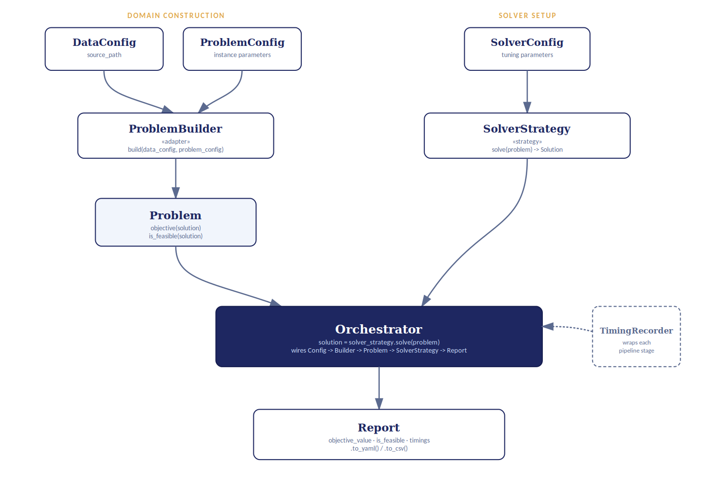
Layer	Lives in	Role
DataConfig / ProblemConfig / SolverConfig	config/	Frozen, self-validating pydantic models. Thin generic bases; concrete use cases subclass them with their own fields.
Problem	domain/problem.py	Immutable domain instance (a graph, a MIP, whatever the problem needs). All mutable state lives on Solution, never here.
ProblemBuilder	domain/builders/	An adapter: DataConfig + ProblemConfig → Problem. One-shot, build once and discard.
Solution	solution/solution.py	Mutable candidate state produced by a SolverStrategy. Its shape is domain-specific.
SolverStrategy	solvers/solver_strategy.py	A complete algorithm: one method, solve(problem) -> Solution. It owns its own loop control and convergence logic.
Report	solution/report.py	Wraps the best Solution, its objective value, feasibility, and timings. Exports to YAML or CSV.
Orchestrator	orchestration/pipeline.py	Wires everything above together for one experiment run, with a TimingRecorder around each stage.

The class hierarchy

The table above is the data flow; this is the same framework as an actual class hierarchy, showing how the abstract pieces the framework ships relate to the concrete pieces one use case, BAP, provides:

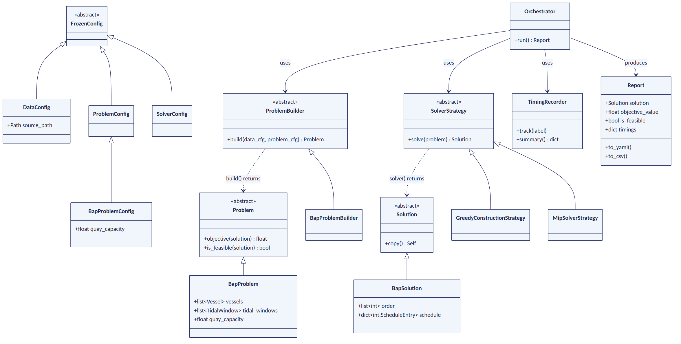
Every arrow into a Bap* class is a solid inheritance arrow, not a dashed one. That’s a direct consequence of using abc.ABC instead of Protocol, more on that below: with abc.ABC the relationship is a real class BapProblem(Problem):, so it’s a genuine is-a relationship the diagram can draw as inheritance. Adding a second use case means adding a second column under the same abstract classes, Citi Bike’s classes would slot in as their own column without touching anything drawn here.

How a run flows end to end

In code, running an experiment is just wiring four things into an Orchestrator and calling .run():

orchestrator = Orchestrator(
    data_config=DataConfig(source_path=instance_path),
    problem_config=BapProblemConfig(quay_capacity=3.0),
    builder=BapProblemBuilder(),
    solver_strategy=MipSolverStrategy(MipSolverConfig(time_limit_seconds=30)),
)
report = orchestrator.run()
print(report.objective_value, report.is_feasible)

Swapping the exact MIP for the greedy heuristic is a one-line change, solver_strategy=GreedyConstructionStrategy(), and nothing else in the pipeline needs to know or care. That one-line swap was the entire point of the exercise: the flexibility my users wanted is now a config change, not a rewrite.

Design principles behind the code

A few conventions carry the weight of keeping this maintainable as it grows, written up in the repo’s docs/python.md:

• One class per file, filename mirrors the class name. The object graph is navigable without an IDE index.

• Explicit abc.ABC inheritance over typing.Protocol. This one needs unpacking if you haven’t run into Protocol before. Python has two ways to define “a class that satisfies this interface”:

  # typing.Protocol: structural typing. No inheritance anywhere, just a
  # matching method signature is enough to count as a SolverStrategy.
  class SolverStrategyProto(Protocol):
      def solve(self, problem: Problem) -> Solution: ...
  
  class MySolver:                       # never mentions SolverStrategyProto
      def solve(self, problem): ...     # satisfies it anyway, implicitly
  
  # abc.ABC: nominal typing. The relationship has to be written down.
  class SolverStrategy(ABC):
      @abstractmethod
      def solve(self, problem: Problem) -> Solution: ...
  
  class MySolver(SolverStrategy):       # explicit, visible right here
      def solve(self, problem): ...
  

  With Protocol, a class becomes a SolverStrategy just by having a method with the right name and signature, nothing in the code ever says so directly, you’d have to go looking to find every class that counts. With abc.ABC, class MySolver(SolverStrategy) says it plainly, and if MySolver forgets to implement solve(), Python raises a TypeError the moment you try to instantiate it, not later when something calls .solve() and gets a confusing failure. For a framework meant to be extended with new use cases over time, I’d rather have that relationship spelled out and fail fast than rely on structural matching. That’s also why the class diagram above draws solid inheritance arrows everywhere instead of dashed ones, abc.ABC gives you a real is-a relationship to draw.

• Pydantic for boundaries, dataclasses for internals. Anything validating external input (DataConfig, ProblemConfig, SolverConfig) is a frozen pydantic model. Anything that’s just internal plumbing (Solution, domain objects) is a plain @dataclass. Pydantic is for validation, not for object plumbing.
• No premature abstraction. Three similar lines beat a shared helper written for a variation that doesn’t exist yet. Two concrete instances of this further down: Citi Bike’s builder takes the framework’s base ProblemConfig directly instead of getting its own subclass, because every parameter it needs already lives in the CSV, there was nothing left to add. And GreedyConstructionStrategy has no SolverConfig subclass at all, in either use case, because it has no tunable parameters, a config class with zero fields would exist only to satisfy a pattern, not a need.
• The object lifetime rule. Before passing an object somewhere, check how far it actually needs to travel. A DataConfig goes to its Builder and no further. Problem is the one exception, shared between Orchestrator and SolverStrategy, because both genuinely need it.

That last one is really the same lesson as the framework’s origin story, just applied at the level of individual objects instead of the whole codebase: don’t let something’s reach exceed what it actually needs.

This separation pays off directly in testing too. Framework-level tests exercise the mechanics (does the pipeline wire correctly, does timing get recorded) against small fakes that don’t know about any real domain. Use case tests exercise real domain logic (does the schedule decode correctly, is the objective computed right) with small, hand-crafted instances. Neither kind of test needs to know about the other.

Use Case 1: Berth Allocation Problem

The problem

A single continuous quay of length quay_capacity. Vessels arrive over time, and each one needs a certain length of quay for a certain number of hours of processing. Several vessels can be alongside at once, as long as their combined length never exceeds the quay’s capacity at any instant. The catch is that a vessel can only actually depart during one of several periodic tidal windows, if processing finishes between windows, the vessel keeps occupying quay space until the next window opens. The objective is to minimize the sum of every vessel’s completion (departure) time.

This is a published benchmark from Ernst, Oğuz, Singh, and Taherkhani’s 2017 paper on mathematical models for berth allocation in dry bulk terminals, not something I invented, which made it a convenient stand-in: realistic combinatorial structure, an existing exact formulation to validate against, and no connection to my actual work problem.

To make the mechanics concrete, here’s a tiny 3-vessel instance decoded into a schedule:

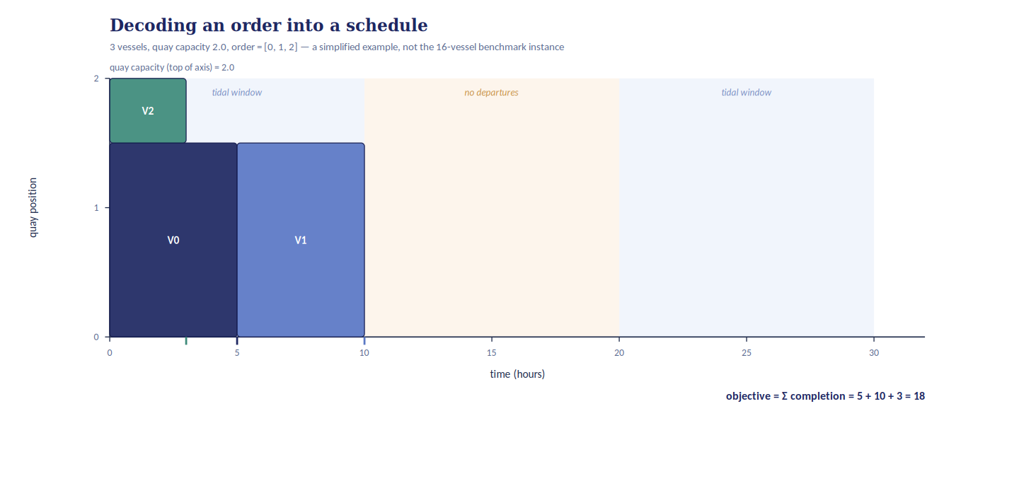
Vessel 0 and vessel 2 share the quay concurrently between time 0 and 3, since their combined length fits under capacity. Vessel 1 has to wait for vessel 0 to clear before it can start, and its completion lands exactly on the boundary of the first tidal window. That snapping behavior, and the concurrent-sharing behavior, are the two things that make this problem more interesting than plain job scheduling.

The data

BapProblemBuilder reads an instance CSV with Vessels / Begin / End / Processing / Length / Arrival rows. The quay capacity itself isn’t in the instance file, it’s constant at 3.0 across every published instance in the benchmark, so it lives on BapProblemConfig instead of the data file. The repo carries one curated 16-vessel instance from the published 900-instance archive.

The solvers

All strategies decode a vessel processing order into a concrete schedule through a shared scheduler.decode() function: serial schedule generation, placing each vessel in order at the earliest feasible time and quay position, snapping its completion to the next tidal window. What differs between strategies is how they search over orders.

• GreedyConstructionStrategy builds earliest-arrival-first, then descends to a local optimum via first-improvement adjacent swaps. No tunable parameters.
• MipSolverStrategy solves the exact MIP from the Ernst et al. paper via pulp and CBC, one-shot to optimality or a time limit. This is the only strategy that needs the optional bap extra, the core framework itself stays solver-library-agnostic.

(The repo also ships a TabuSearchStrategy over the same swap neighborhood with an aspiration criterion and a tabu tenure; I’m leaving it out of this walkthrough for length, the README covers it.)

Running both on the 16-vessel instance:

Strategy	Objective	Solve time
Greedy construction + local search	1675.00	0.004s
Exact MIP	1668.00	13.12s

The exact solve finds an objective about 0.4% better, at roughly 3000 times the compute cost. Neither number is the point, really, the point is that getting both numbers took changing one constructor argument, not two separate scripts.

Use Case 2: Citi Bike Station Rebalancing

The problem

A fixed fleet of bikes spread across a set of stations, each with a fixed number of docks. Given predicted pickup and dropoff demand per station for an upcoming period, decide a target bike count per station, redistributing the existing fleet rather than adding or removing bikes, that minimizes predicted lost demand. A stockout happens when a station has fewer bikes than predicted pickups; a dockout happens when it has fewer free docks than predicted returns. The scope is deliberately narrow: this is the allocation decision only, not the truck routing that would physically move the bikes.

Here’s the mechanic on a tiny 2-station example, redistributing 5 bikes total:

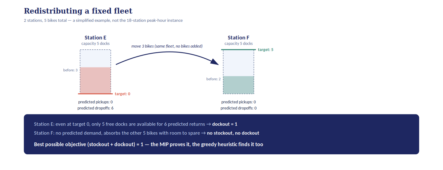
Station E has capacity 5 but 6 predicted dropoffs, so even after moving every one of its bikes out to make room, it’s still one dock short. Station F has no predicted demand at all, so it can absorb the rest of the fleet with room to spare. The best achievable objective here is 1, and it’s unavoidable given the numbers, no reallocation fixes a capacity shortfall that big.

The data

CitibikeProblemBuilder reads a CSV of station_id, name, capacity, current_inventory, predicted_pickups, predicted_dropoffs rows. Every parameter for this problem lives in the CSV itself, so unlike BAP there’s no use-case-specific ProblemConfig, the builder takes the framework’s base config directly. The repo’s curated instance is 18 real Jersey City stations during a weekday morning peak window, built from NYC’s public Citi Bike trip data plus a live GBFS snapshot for station capacity and current inventory.

The solvers

• GreedyConstructionStrategy starts from current inventory, which is trivially feasible, then descends via first-improvement single-bike transfers between stations.
• MipSolverStrategy solves exactly: an integer target per station bounded by capacity, continuous stockout and dockout variables, one fleet-conservation constraint, via pulp and CBC.

The demo script chains four consecutive rebalancing periods, each one warm-started from wherever the previous period’s solved allocation left the stations, which is the more realistic way this decision actually gets made day over day:

Period	Greedy objective	Greedy time	MIP objective	MIP time
1	0.00	0.011s	0.00	0.012s
2	0.00	0.003s	0.00	0.010s
3	0.00	0.003s	0.00	0.010s
4	0.00	0.003s	0.00	0.010s

Both strategies land on objective 0 every period here, this particular curated instance has generous dock capacity relative to demand, so all predicted demand gets covered. That’s not a flaw in the demo, it’s actually a nice cross-check: an exact solver and a simple greedy heuristic agreeing across four chained, warm-started periods is reasonable evidence that both are implemented correctly. A busier time window or a smaller station set would produce a non-zero objective and a more visible gap between the two, the data README has the regeneration script for that if I want a sharper demo later.

What This Bought Me

None of this changes what problem gets solved or how good the answer is, a MIP is still a MIP whether it sits inside a tidy framework or a single script. What changed is everything around the solving: trying a new solver strategy is a constructor argument, adding a new use case is five interfaces instead of a fresh script, and the framework-level tests give me confidence that the plumbing works before I’ve written a single line of domain logic. That’s the flexibility I was missing when I started, and it turned out the fix wasn’t a better formulation, it was better design around the formulation I already had.

If you want to poke at it yourself, the repo is at github.com/hovinh/optimization-framework, with both use cases runnable end to end via scripts/run_bap_poc.py and scripts/run_citibike_poc.py.