An education toolkit to illustrate Dynamic Time Warping algorithm
in Blog
Prerequisite: recursion concept, Python programming language.
Code: Github
Sequential data is any data whose order matters, that consequently, renders its behaviour predictable to certain extent. From stock price chart, smart watch’s heart rate monitor, to next-seven-day humidity levels in weather forecast, we are basically surrounded by this form of data. As the old saying goes, “History repeats itself”, richly informative time component in sequential data allows pattern discovery in the past, trace monitoring in the presence, and trend prediction in the future.
In manufacturing process, the engineers are interested in quality control chart (Fig. 1): a graphic monitors a product’s specific attribute measurement within a predefined specification; any data point deviates beyond threshold limit indicates a machine health or product issue, thus we take immediate action. It’s straightforward to apply such method on summary statistics data, but to take the advantage of sequential data, time series in particular, a finer granularity is required. Dynamic Time Warping (DTW) algorithm is a good candidate for such problem, in which given a pair of varying-length time series, one can obtain a control-chart-appropriate numerical metric that quantifies the time series similarity.
This post will explain the algorithm in great detail, that not only developers can confidently modify as will to fit in their need, but also benefit users with visual aid to demonstrate DTW’s capacity. When applicable, I also comment on possible improvements and other applicable usages.
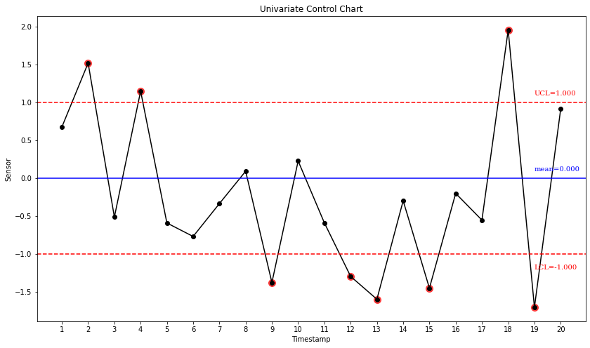 Fig. 1. A typical Control Chart looks similar to the above. Each data point represents for one product item; those whose sensory values go beyond the Upper/Lower Control Limit deemed Out-Of-Control and worth inspecting. In general, given a sufficient amount of data, a 3-sigma control limit should be a good boundary between well-behaved and outlier ones.
Just A Glimpse
What DTW offers can best be illustrated in Fig. 2. On the left, we have two time series that closely share a same pattern, except for the first one slightly longer at the beginning. On the right, every single point in the first time series has at least one mapping to the other, and vice versa. Notice the top right chart, it shows the summation of mapping’s value at each timestamp of the first time series.
To obtain such outcome, DTW’s objective is defined as follows: Given two time series with various lengths, \(s_1\) and \(s_2\), we seek for way to quantify the difference between the two. Interestingly, while retaining that goal, we can state this question in an optimization form: “How can one transform a times series \(s_1\) to time series \(s_2\), with minimal change?”
With that in mind, the algorithm is designed to return a set of mappings that represent the transformation, guaranteedly that the total absolute gap of those mapped point pairs is optimally the lowest. This total gap can leverage into a distance metric. The lower the effort to transform, the smaller the metric’s value, the more \(s_1\) similar to \(s_2\). A bonus is that DTW is symmetrical, implying the transformation from \(s_2\) to \(s_1\) must return the same outcome.
Please bear with me while paving the way for the novel idea of DTW. As such, let’s take a detour to Fibonacci sequence and visit the concept of recursion.
 Fig. 2. Left chart: Two time series \(s_1\) and \(s_2\). Right chart: There is at least one mapping between elements of the two time series. The top bar chart shows the total absolute gap of these mappings, at each timestamp of \(s_1\).
Fibonacci Sequence
Fibonacci sequence is a sequence of numbers, simply such that each number is the sum of the two preceding ones, starting from 0 and 1. It is formally stated in the below recursive formula: \[\begin{cases} F(0) = 0\\ F(1) = 1\\ F(n) = F(n-1) + F(n-2) & \text{for } n \ge 2 \end{cases}\]
The above definition can straightforwardly be translated to an equivalent runnable pieces of code:
# compute Fibonacci number based on recursion
def Fibonacci(n):
    if ((n < 0) or (type(n) != int)):
        raise ValueError('Argument n only accepts a positive integer.')

    if (n == 0):
        return 0
    if (n == 1):
        return 1
    return Fibonacci(n-1) + Fibonacci(n-2)
print (Fibonacci(n=4))
At first glance this recursive implementation returns outcome instantly, but it’s getting noticably low starting from \(n=35\) onwards. Unfolds the execution, as illustrated in The Fig. 3., you can notice \(F(n=2)\) is computed twice. As \(n\) grows bigger, more Fibonacci numbers recomputed and unavoidably leads to an absurd amount of wasted computational power. What if, we can compute every number only once?
Gladly, you can always turn a recursive function into an iterative process, i.e. a loop and a stack (optional)(1)(2).
# compute Fibonacci number in iterative manner
def Fibonacci(n):
    if ((n < 0) or (type(n) != int)):
        raise ValueError('Argument n only accepts a positive integer.')

    Fibonacci = [0, 1] # F(0) = 0; F(1) = 1
    for i in range(2, n+1, 1):
        Fibonacci_i = Fibonacci[i-1] + Fibonacci[i-2] # F(n) = F(n-1) + F(n-2)
        Fibonacci.append(Fibonacci_i)

    return Fibonacci[n]
print (Fibonacci(n=4))
We create a 1-D array to store all computed Fibonacci numbers and a means to quickly retrieve number using the array index - the \(i\)th element in the array contains the value of \(F(n=i)\). Start with \(i=0\) and \(i=1\) as building blocks, the followings step flows naturally to compute \(F(2)\), \(F(3)\), …, up to \(F(n)\). The last value of the array is the Fibonacci number of interest. Now, even with \(F(n=1000)\), it can be computed in the blink of an eye.
There is certain trade-off that one sacrifices to earn this efficiency. On one hand, each Fibonacci number computed once and the amount of computation increase linearly with \(n\) increases by one unit - not the best, but a computational complexity most algorithms dream of. On the other hand, it takes more time to “decipher” the implementation, say, why a loop and an array exist? The abstraction and straightforwardness of recursion is replaced by a slightly cryptic code that lifts off the wasted duplication in the computing process.
DTW, to no surprise, designed in this manner and inevitably makes people confusing rather than dumbfounded, as it should be, when they have first look at the implementation. However, Fibonacci is a simplified version of DTW, and if you still follow me till now, I believe we are ready to tackle it!
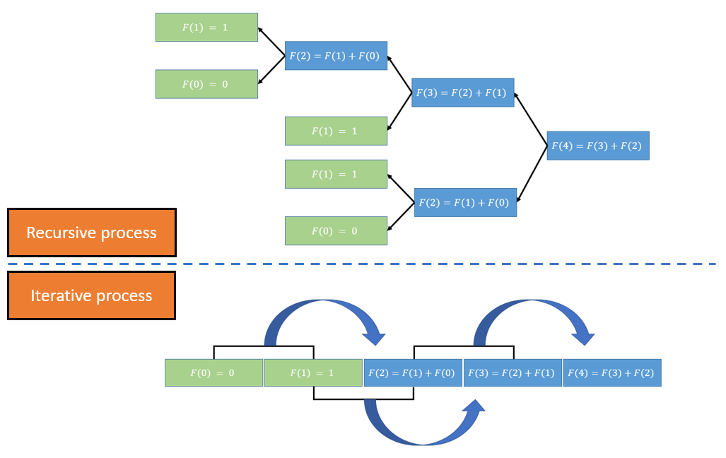 Fig. 3. Two approaches to compute Fibonacci sequence. Top: Recursive process - each number is computed backward by calling the function of two preceding ones, till \(n=0\) and \(n=1\), then forward the values back to the original call. Bottom: Iterative process - An array stores computed values with \(i=0\) and \(i=1\) as building blocks; it expands the length linearly to the value of \(n\).
Still Fibonacci, but in 2-D: Dynamic Time Warping algorithm
“How can one transform a times series \(s_1\) to time series \(s_2\), with minimal change??”
Let’s align on the terminology prior to formulate this objective:
- An element \(s_1^i\) is the value of time series \(s_1\) at the timestamp \(i\)th.
- Time series \(s_1\) and \(s_2\) have \(m\) and \(n\) elements, respectively.
- A mapping \((s_1^i, s_2^j)\) is a connection established between two elements of time series \(s_1\) and \(s_2\). In DTW context, we call this a transformation, indicating that \(s_1^i\) can change an amount of \((s_2^j-s_1^i)\) to partially turn \(s_1\) into \(s_2\), and vice versa. Note that every element strictly has at least one mapping to the other time series.
- Each mapping \((s_1^i, s_2^j)\) has a weight \(w(s_1^i, s_2^j)\), computed by the absolute gap of the two elements: \(\lvert(s_2^j-s_1^i)\rvert\). In DTW context, we call this a change.
Formally, our objective states:
In plain English, we would like to pick a set of mappings whose summation of weights is minimum, under the constraint that:
- each elements must have at least one mapping connects to it (condition 1 and 2).
- there is no crossover between any mappings (condition 3).
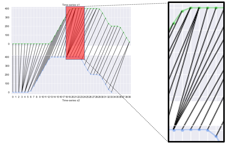 Fig. 4. Each element in a time series is connected to at least one element in the other time series.
The above formularizing attempt is not to scare readers away, but to emphasize that the constrainsts must be acknowledged and held, in order for the algorithm to work. As a bonus, I conveniently show that linear programming is an alternative way to solve this optimization problem.
As stated earlier and now I shall clarify, Fibonacci sequence is similar to DTW: both can be solved using an algorithmic technique, namely Dynamic Programming(3). To determine a problem solvable in this manner, it must have the following attributes:
- Optimal subproblems: a large problem is the combination of similar subproblems, if, once whose optimal solutions obtained, can therefore help derive the optimal solution for the large problem.
- Overlapping subproblems: the subproblems are recursively repeated multiple times.
The fact that Fibonacci sequence is defined in recursion show that it intrinsically contains an overlapping subproblems. And despite it’s true that there is no pursuit of optimality, but \(F(n)=F(n-1) + F(n-2)\) shows the large problem can be solved once the subproblems solved. The second approach - iterative process - is its Dynamic Programming implementation.
With no more delay, here comes the straightforward, recursive version of the DTW algorithm:
def DTW(s1, i, s2, j):
    # s1, s2: 1-D array.
    # building blocks
    infinity =  float('Inf')
    if ((i <= 0) or (j <= 0)):
        return infinity

    new_weight = abs(s1[i] - s2[j])
    if ((i==1) and (j==1)):
        return new_weight

    # Overlapping subproblems
    cumulative_weights = ([
        DTW(s1, i, s2, j-1),     # immediate adjacent mapping is (s1[i], s2[j-1])
        DTW(s1, i-1, s2, j),     # immediate adjacent mapping is (s1[i-1], s2[j])
        DTW(s1, i-1, s2, j-1),   # immediate adjacent mapping is (s1[i-1], s2[j-1])
    ])

    # Optimal subproblems
    cumulative_weight = min(cumulative_weight) + new_weight
    return cumulative_weight

s1 = [1, 2, 3, 3, 5]
s2 = [1, 3, 6]
s1_last_index = len(s1) - 1
s2_last_index = len(s2) - 1
print (DTW(s1=s1, i=s1_last_index, s2=s2, j=s2_last_index))
Constraint 1: each elements must have at least one mapping connects to it.
Constraint 2: there is no crossover between any mappings.
The first constraint implies that, regardless of whatever the optimal set of mappings is, it must always include \((s_1^{i=1}, s_2^{j=1})\) and \((s_1^{i=m}, s_2^{j=n})\), which are the building block and guaranteed end in Fig. 5. This constraint, combining with the second “no-crossover” rule, implies that for any mapping \((s_1^{i}, s_2^{j})\), there are only 3 possibilities of immediate precede mapping, as shown in Middle phase: the possibility with the lowest cumulative_weight is the solution for subproblem, in turn integrated as part of the solution for the big problem. The new_weight is simply \((s_1^{i=1}, s_2^{j=1})\) when the function DTW reaches Beginning phase, \((s_1^{i}, s_2^{j})\) the Middle phase, and \((s_1^{i=m}, s_2^{j=n})\) the Ending phase. Similar to Fibonacci, in recursive form, things need to compute backward, therefore the algorithm starts from Ending phase, to Middle phase then Beginning phase; once reaches the building block, it forwards the values back to the original call.
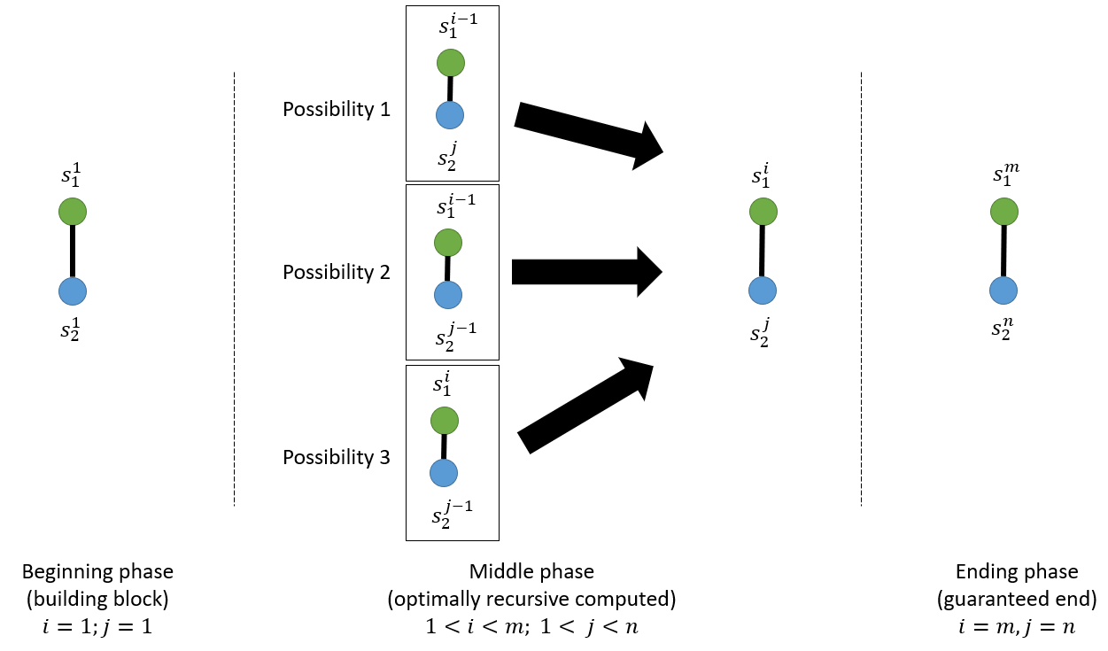 Fig. 5. Breaking up the DTW algorithm into 3 main phases.
There is no wasted computation - duplicated recomputation of an element - in DTW. One can also retrieve the optimal mapping set with additional few lines of code. However, there is certain limit in recursive calls and flexibility to make the algorithm smarter and more efficient. An iterative process will allow you to construct all mapping from the Beginning phase, with certain strategies to embed your opinion of a good mapping, to Ending phase; then later backtracking to retrieve the optimal mappings (notice that there could be more than one optimal solution).
Here is the idea:
- The mapping is encoded as a 2-D matrix (array) \(A\), whose cell \(A_{i,j}\) represents for the mapping \((s_1^{i}, s_2^{j})\).
- You fill up the matrix from left to right, top to bottom. In other words, for every \(i\)th row, you compute the cumulative weight for all mappings between \(s_1^{i}\) and all elements in \(s_2\), using the insights of 3 possibilities. Once filled up, the bottom right cell, \(A_{m,n}\), is the DTW distance.
- To retrieve the optimal mapping, one backtrack from \(A_{m,n}\), again using the 3 possibilities to pick one with the lowest cumulative weight, up till \(A_{1,1}\).
Interested readers can view the implementation here, whereas I simply show an illustration instead.
 Fig. 6. Illustration of DTW algorithm implemented in iterative manner.
I have a mapping, I have a DTW distance. Uh! What’s next?
You have a powerful technique to manipulate time series, of that I’m certain. Its impact can be discussed at two scales: DTW plays a primary or a minimal supporting role in your problem.
Let’s talk about DTW as a primary method. You may encounter the obtained mapping not match well with human intuition, despite its minimum distance. One can impose additional constraint (4), say, an element cannot have more than \(k\) mappings, prioritize 1-1 mapping over n-1, or no long distance mapping, by modifying the strategy to fill up the matrix \(A\). Other DTW variants deal with the accuracy-processing time tradeoff; in general, DTW’s complexity is \(O(n^2)\), with \(n\) is the time series’ length, which becomes costly when \(n\) increases, in terms of both memory and computational power. Instead of one matrix, they employ multiple versions at different sampling scales of \(A\), or a fixed limit on which area to fill in \(A\), provided certain assumptions on the time series input.
However, sometimes DTW is not a good fit. If the noise cannot be distinguished from general trend of the time series, the “Garbage in, Garbage out” principle holds. One should remove noise first, say, time series decomposition, or smoothing/approximating with a linear regression line or a polynomial of choice.
In a bigger picture, DTW’s supporting role can blend in nicely with generic Machine learning problems. Here’s my personal use in the past, but the list surely go on:
- A smart sampling strategy: you have two different-length time series and would like to compare them point-wise? One can perform an asymmetric sampling to transform one time series to have the same length with the other, using the DTW mapping. Example.
- A kernel function: you have a bunch of time series and would like to group them based on similarity? How about K-Means clustering with DTW as kernel to compute the distance between “time series” data points?
- A univariate control chart: we have established a standard process flow, how to monitor the sequential runs to follow the same specification? I would first established a so-called “golden trace” time series, then compute DTW distance of upcoming runs with respect to this trace. Given each run has one numerical value quantifying its deviation from the golden trace, users can employ a 3-sigma control chart for quality control purpose.
And yep, that concludes my sharing on DTW. Hope this post provides you some new insights on this helpful algorithm. Feel free to share with me your thoughts and any feedback on this.
(1) https://stackoverflow.com/questions/531668/which-recursive-functions-cannot-be-rewritten-using-loops
(4) https://www.audiolabs-erlangen.de/resources/MIR/FMP/C3/C3S2_DTWvariants.html