Fourier Transform

02 Jul 2023 in Blog

Fourier Transform is a novel method that is widely used in signal processing. This post to explain the intuition behind its mathematical operations and idea to apply it in machine learning.

Code: Github

Have you ever wondered how a signal can be broken down into its fundamental components? Welcome to the ingenious concept of the Fourier Transform. This transformative technique allows us to express a signal as a sum of basis signals, opening up a world of possibilities for understanding and manipulating data.

By decomposing complex signals into simpler and more interpretable components, we gain a constructive lens through which we can explore their nature. We can manipulate these components at will, observing their influence on the original signal and even transforming the signal itself under controlled conditions. For practitioners of machine learning, the potential of such a method in data analysis is undeniable.

But here’s the real beauty: the power of the Fourier Transform extends far beyond the realm of numbers. It is applicable to a wide range of natural phenomena, from time series and 2D images to audio recordings and higher-dimensional functions.

In this blog post, I will guide you through the Fourier Transform algorithm, explaining its inner workings in an intuitive manner supported by adequate mathematical reasoning. Although we will focus on univariate time series for the sake of brevity, the concepts and principles discussed can easily be extended to higher-dimensional domains.

By the end of this journey, you will not only have a thorough understanding of the Fourier Transform but also gain insights into its diverse applications and ideas for your next project.

• Updated Jul/2023: modify normalization terms in computing \(C_n\) and \(D_n\). Thanks to @chanlenger’s comment.

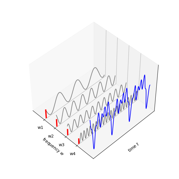Fig. 1. The blue signal \(f(t)\) that is expressed in time axis \(t\) can be deconstructed into a set of sine waves with varying frequencies (black waves). These waves have their influence, or contribution to \(f(t)\), quantifiable to a numerical quantity that can be displayed on the frequency axis \(w\).

Background knowledge

Before diving into the inner workings of the algorithm, it’s crucial to establish and demonstrate certain concepts and characteristics.

At the heart of the Fourier Transform lies the sinusoid, a fundamental building block. A sinusoid is a smooth and repetitive oscillation, symmetrically fluctuating around a central value. It can be represented mathematically as a sine or cosine function. Three key parameters define a sinusoid: amplitude (\(A\)), angular frequency (\(w\)), and initial phase (\(-\theta^\prime\)).

In Figure 2, we observe three sinusoids \(g(t) = Acos(-\phi^\prime+wt)\) with varying parameter values. The amplitude (\(A\)) determines the maximum height of the oscillation, as seen in the example where the blue wave extends four times further than the red and green waves. The initial phase (\(-\theta^\prime\)) indicates the starting point of the wave, with \(-\theta^\prime=0\) representing the wave’s peak and \(-\theta^\prime=\pi\) radian representing the wave’s trough. Additionally, if the wave takes \(T\) seconds to complete one full cycle (where a complete cycle is 360 degrees or \(2 \pi\) radians), then the frequency (\(w=2 \pi/T\)) represents the rate of radians per second. Therefore, both \(w\) and \(-\theta^\prime\) are essential in determining the waveform’s position within its cycle at any given moment in time.

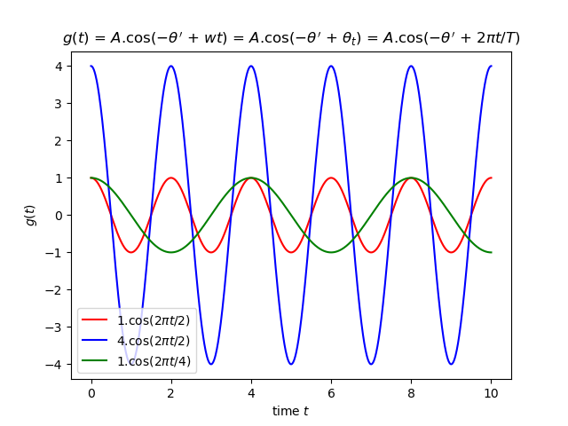Fig. 2. Three sinusoids illustrate the effect in wave shape that is determined by the three parameters amplitude \(A\), angular frequency \(w\), and initial phase \(-\theta^\prime\).

If we denote \(\phi_t = wt\), we can reorganize the sinusoid as follows: \[\hspace{10pt} g(t) = A cos (-\phi^\prime + wt) = A cos(-\phi^\prime + \phi_t ) = A cos(\phi_t -\phi^\prime)\]

We then proceed to show that any sinusoid can be expressed as a linear combination of a sine and cosine function in the form: \[\hspace{10pt} g(t) = A cos(\phi_t -\phi^\prime) = C cos\phi_t + D sin\phi_t\]

Given the trigonometric identity \(cos(\alpha - \beta) = cos\alpha cos\beta + sin\alpha sin\beta\), we have \[\hspace{10pt} A cos(\phi_t -\phi^\prime) = A (cos\phi_t cos\phi^\prime + sin\phi_t sin\phi^\prime) = [A cos\phi^\prime]cos\phi_t + [A sin\phi^\prime]sin\phi_t\]

Plug this back in \(g(t)\), it then shows \[\hspace{10pt} \boldsymbol{[A cos\phi^\prime]}cos\phi_t + \boldsymbol{[A sin\phi^\prime]}sin\phi_t = \boldsymbol{C} cos\phi_t + \boldsymbol{D} sin\phi_t\]

As a result, we have \(\boldsymbol{C = A cos\phi^\prime}\) and \(\boldsymbol{D = A sin \phi^\prime}\). Furthermore, given \(sin^2 \phi^\prime + cos^2 \phi^\prime = 1\), we have \(\boldsymbol{A=\sqrt{C^2+D^2}}\) and \(\boldsymbol{\phi^\prime=arctan(D/C)}\). This interestingly implies one can represent a sinusoid with either pair of parameters: the amplitude (\(A\)) and initial phase (\(\phi^\prime\)), or the amplitude (\(C\)) of a cosine and amplitude (\(D\)) of a sine whose summation construct the same sinusoid.

Indeed, Fig. 3. show that for any sinusoid \(A cos(\phi_t -\phi^\prime)\) with known \(A\) and \(\phi^\prime\), one can compute the counterpart pair \(C\) and \(D\) and the visualization intuitively verifies that mathematical property.

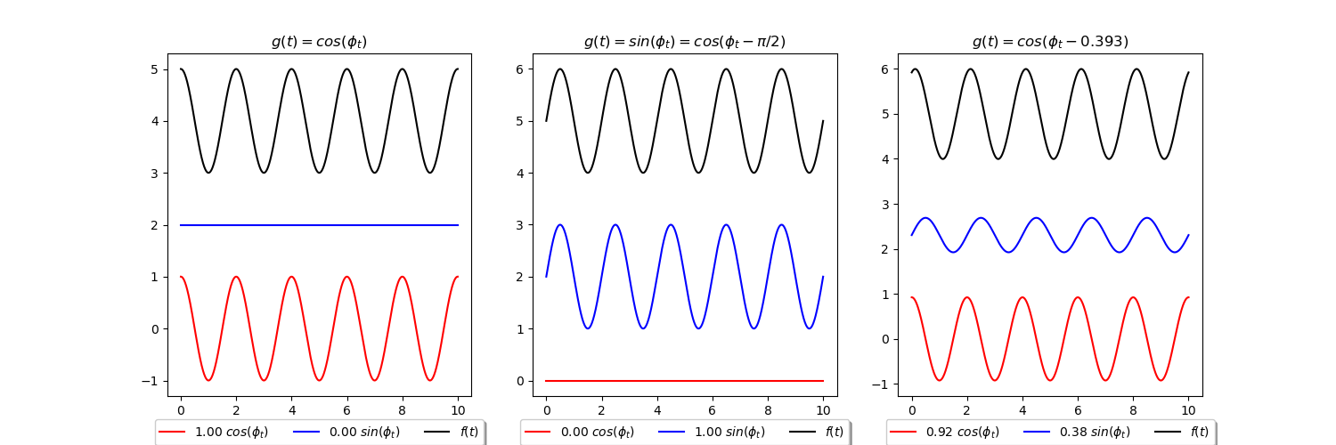Fig. 3. Sinusoids with three different parameter set \([A=1, \phi^\prime=0 \text{ rad}]\), \([A=1, \phi^\prime=-\pi/2 \text{ rad}]\), \([A=1, \phi^\prime=0.393 \text{ rad}]\), displayed in black, and their decomposition to sine and consine functions, blue and red respectively.

Moving forward, let’s introduce the concept of sinusoidal basis functions, which form a family of functions capable of approximating any function \(f(t)\). It’s important to note that the term “any function” encompasses a broad range of functions, extending beyond sinusoids alone.

Consider an arbitrary function \(f(t)\) with an input time argument \(t \in [0, T]\). To begin approximating this function using sinusoidal basis functions, we start with the first basis function. Its angular frequency is denoted as \(w_1 = 2\pi/T\) (rad/s), meaning that it has a period of \(T\) seconds. We refer to \(w_1\) as the fundamental frequency.

However, to achieve a more accurate approximation, we need to incorporate additional complex functions known as harmonics. These harmonics are multiples of the fundamental frequency \(w_1\) and are represented by successive values of \(n \in \mathbb{N}\), where \(\mathbb{N}\) denotes the set of natural numbers:

\(\hspace{60pt} w_1 = 1 \times w_1,\)
\(\hspace{60pt} w_2 = 2 \times w_1,\)
\(\hspace{60pt} w_3 = 3 \times w_1,\)
\(\hspace{60pt} ...\)
\(\hspace{60pt} w_n = n \times w_1\)

Therefore, the approximation of a function \(f(t)\) with sinusoidal basis functions would be \[f(t) = \sum_{n \in \mathbb{N}} A_n cos(w_nt - \phi^\prime_n) = \sum_{n \in \mathbb{N}} g_n(t)\]

And because a sinusoid \(g_n(t)\) can be expressed as a linear combination of a sine and cosine function, hence \[f(t) = \sum_{n \in \mathbb{N}} C_n cos(w_nt) + D_n sin(w_nt)\]

Lastly, by this construction, we can leverage on the orthogonal properties of basis function to obtain Fourier coefficients \(C\) and \(D\) in the formula presented earlier for each sinusoidal component. Suppose we aim to determine the coefficient \(C_m\) of the harmonics, where \(w_m = m \times w_1\). We can accomplish this by multiplying the function \(f(t)\) by consine (\(cos(w_mt)\)) and integrating over \(t\) within the range of \(-T/2\) to \(T/2\): \[\int_{-T/2}^{T/2} f(t) cos(w_mt)dt = \int_{-T/2}^{T/2}[\sum_{n \in \mathbb{N}} C_ncos(w_nt) + D_nsin(w_nt)] cos(w_m)dt = \sum_{n \in \mathbb{N}} C_n \int_{-T/2}^{T/2} cos(w_nt) cos(w_m)dt + \sum_{n \in \mathbb{N}} D_n \int_{-T/2}^{T/2}sin(w_nt) cos(w_m)dt\]

Despite its intimidating expansion, because any pair \(\boldsymbol{sin(w_nt)cos(w_mt) = 0, (\forall m, n)}\) and \(\boldsymbol{cos(w_nt)cos(w_mt) = 0, (\forall m \neq n)}\), we can simplify the equation into \[\int_{-T/2}^{T/2} f(t) cos(w_mt)dt = C_m\int_{-T/2}^{T/2} cos(w_nt) cos(w_mt) dt = C_m\int_{-T/2}^{T/2} cos^2(w_mt) dt = C_m \frac{T}{2}\]

Because all variables are known except for \(C_m\), hence \[C_m = \frac{2}{T} \int_{-T/2}^{T/2} f(t) cos(w_mt) dt\]

Likewise, by multiplying \(f(t)\) by \(sin(w_mt)\), we obtain \[D_m = \frac{2}{T} \int_{-T/2}^{T/2} f(t) sin(w_mt) dt\]

To address any doubts you may have regarding the simplification step, allow me to provide a clearer explanation with the help of Figure 4. This figure demonstrates two waves in each row, with frequencies that are harmonics of a fundamental frequency \(w_1\), along with an example of their multiplication along the time axis.

Let’s consider the first row as an example, which consists of the waves \(\boldsymbol{sin(\phi)}\) and \(\boldsymbol{cos(2\phi)}\). The integral of their multiplication, denoted as \(\boldsymbol{\int_{-T/2}^{T/2} sin(\phi) cos(2\phi) dt}\), can be visualized as the summation of the shaded areas within the time interval \([-T/2, T/2] = [-5, 5]\). Upon observation, you’ll notice that the positive and negative sides symmetrically cover the same amount of area, resulting in a total sum of zero. This same principle applies to the second example, where \(\boldsymbol{\int_{-T/2}^{T/2} cos(\phi) cos(2\phi) dt = 0}\).

Furthermore, in the case of \(\boldsymbol{\int_{-T/2}^{T/2} cos^2(\phi) dt} = T/2\), which is depicted in the figure, the integral evaluates to \(T/2\). Once again, this can be verified by examining the figure.

Although these examples are provided for clarity, the underlying principle holds true for other similar pairs with varying frequencies, as long as their frequencies maintain a harmonic relationship.

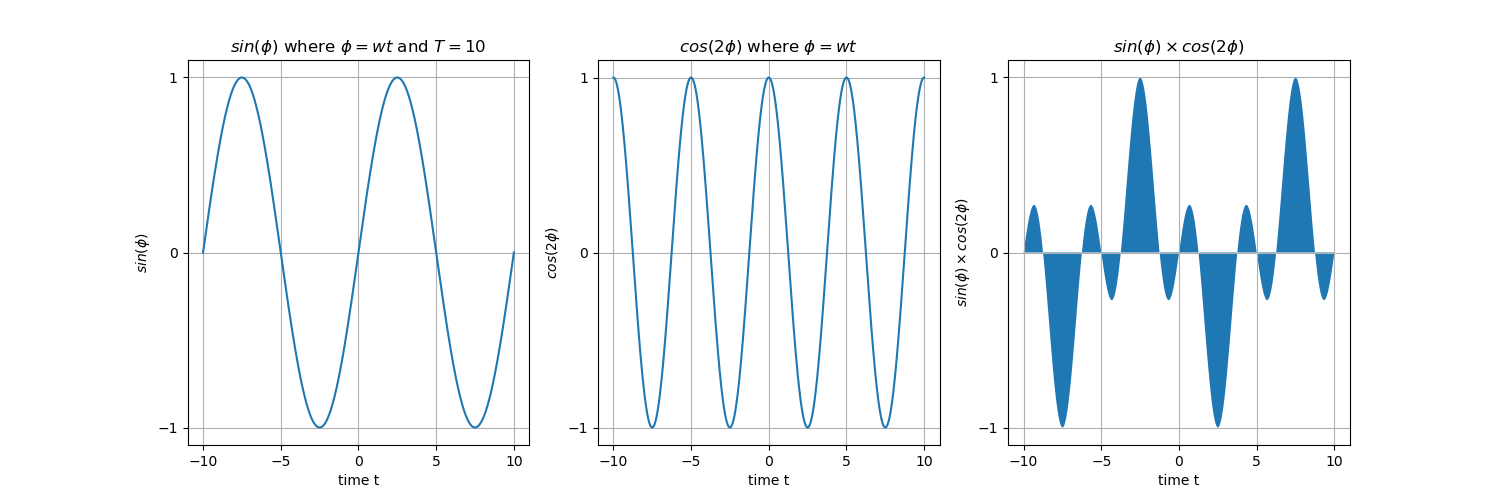
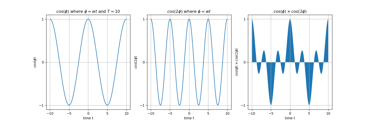
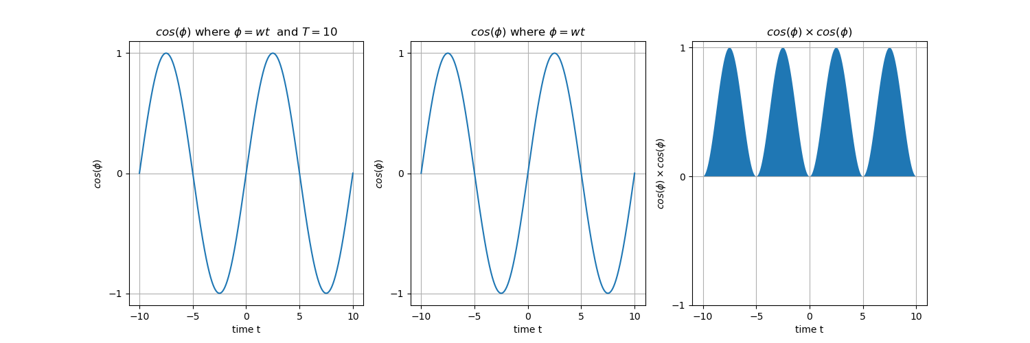Fig. 4. Row 1: The integral of any \(sin(nwt) \times cos(mwt)\) is zero. Row 2: The integral of any \(cos(nwt) \times cos(mwt)\) is zero. Row 3: The integral of any \(cos^2(nwt)\) is \(\frac{T}{2}\).

Discrete Fourier Transform Algorithm

Now that we have established the necessary background, let us proceed with the algorithm. In this context, the term “discrete” implies that the basis function takes whole-number multiples of a fundamental frequency.

Figure 5 vividly illustrates the Fourier Transform in action when applied to a synthetic curve \(f(t)\). This curve is deconstructed into 500 cosine waves, where the fundamental frequency \(w_1\) and the harmonics \(w_2\) exhibit significant amplitudes and higher frequencies \(w_3, w_4, ..., w_{500}\) have amplitudes approaching zero. By summing these 500 waves, we can achieve a nearly perfect reconstruction \(f^\prime(t)\).

Furthermore, by plotting each frequency \(w_n\) from the sinusoidal basis functions on the x-axis and their corresponding amplitudes \(A_n\) on the y-axis, we can form the amplitude spectrum of the curve \(f(t)\). This spectrum reveals the frequencies that contribute the most to the shape of \(f(t)\), with the expected prominence of the fundamental frequency \(w_1\) and the harmonic \(w_2\).

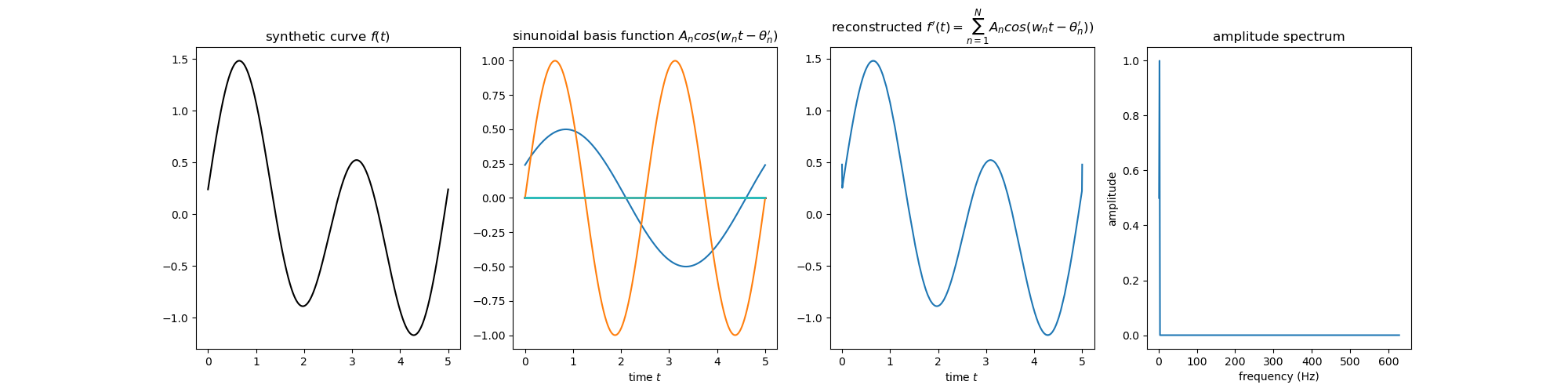Fig. 5. Column 1: A synthetic curve \(f(t)\). Column 2: Applying Fourier transform and compute the sinusoidal basis functions that approximate \(f(t)\) in form of \(A_n cos(w_nt - \phi^\prime_n), \forall 1 \leq n \leq 500\). Column 3: Reconstruct \(f^\prime(t)\) using the formula \(\sum_{n=1}^\mathbb{500} A_n cos(w_nt - \phi^\prime_n)\). Column 4: The plot of \(A_n\) to see the contribution of each frequency \(w_n = n \times w_1\) in the basis functions.

I use the code below to produce the figure.

n_samples = 1000
x, ft, T = generate_curve_ft(n_samples)
fundamental_frequency = 2 * math.pi / T
n_frequencies = 500
freqs, Cs, Ds = fourier_transform(fundamental_frequency, n_frequencies, n_samples)
As, thetas, sinusoids = compute_sinusoidal_basis_function(Cs, Ds, x)
reconstructed_ft = np.sum(sinusoids, axis=0)

f, (ax0, ax1, ax2, ax3) = plt.subplots(nrows=1, ncols=4, figsize=(20, 5))

# synthetic curve ft
ax0.plot(x, ft, color='black')
ax0.set_title(r'random function $f(t)$')
ax1.set_xlabel(r'time $t$')

# obtain sinusoidal basis function
for sinusoid_n in sinusoids:
    ax1.plot(x, sinusoid_n)
ax1.set_title(r'sinusoidal basis function $A_n cos(w_nt - \theta^\prime_n)$')
ax1.set_xlabel(r'time $t$')

# reconstructed functions
ax2.plot(x, reconstructed_ft)
ax2.set_title(r'reconstructed $f^\prime(t) = \sum_{n=1}^N A_n cos(w_nt - \theta^\prime_n))$')
ax2.set_xlabel(r'time $t$')

# amplitude spectrum
ax3.plot(freqs,As)
ax3.set_xlabel('frequency (Hz)')
ax3.set_ylabel('amplitude')
ax3.set_title('amplitude spectrum')
plt.show()

Firstly, I create a synthetic curve \(f(t)\) by combining the values of two arbitrary sine waves. However, I deliberately selected their frequencies in such a way that the pattern of \(f(t)\) repeats every \(T=5\) seconds. It’s important to note that this periodicity is merely an example, and you are free to substitute it with any arbitrary non-periodic function of your choosing.

def generate_curve_ft(n_samples):
    T = 5
    x = np.linspace(0, T, n_samples)
    sin_y1 = get_sinewave_y(1, 2.5, 0, x)
    sin_y2 = get_sinewave_y(0.5, 5, 0.5, x)
    ft = plus_waves(sin_y1, sin_y2)

    return x, ft, T

def plus_waves(Y1, Y2):
    return Y1 +  Y2

Next, in order to approximate the curve \(f(t)\), I have chosen to employ 500 sinusoidal basis functions. These functions are designed to capture the essence of \(f(t)\) by utilizing a fundamental frequency \(w_1 = 2 \pi/T = 2\pi/5\). Consequently, we can determine the frequencies of the subsequent basis functions as follows: \(w_2 = 2 \times w_1 = 4\pi/5\), \(w_3 = 3 \times w_1 = 6\pi/5\), and so on. Each frequency \(w_n\) is obtained by multiplying the fundamental frequency \(w_1\) by the respective harmonic index \(n\).

By leveraging the orthogonal properties of these basis functions, we can calculate the coefficients \(C_n\) and \(D_n\) by multiplying \(f(t)\) with the cosine (\(cos(w_nt)\)) and sine (\(sin(w_nt)\)) of the respective frequencies \(w_n\). Through this process, the curve is effectively decomposed into multiple sine and cosine waves, capturing its various components.

def fourier_transform(fundamental_frequency, n_frequencies, n_samples):
    freqs, Cs, Ds = list(), list(), list()


    for n in range(1, n_frequencies+1, 1):
        harmony_freq_n = n * fundamental_frequency
        T_n = 2*math.pi/harmony_freq_n
        cosine_wave_freq_n = get_cosinewave_y(A=1, T=T_n, theta=0, x=x)
        C_n = compute_integral_of_wave_multiplication(ft, cosine_wave_freq_n, n_samples)

        sine_wave_freq_n = get_sinewave_y(A=1, T=T_n, theta=0, x=x)
        D_n = compute_integral_of_wave_multiplication(ft, sine_wave_freq_n, n_samples)

        freqs.append(harmony_freq_n)
        Cs.append(C_n)
        Ds.append(D_n)

    return freqs, np.array(Cs), np.array(Ds)

def get_sinewave_y(A, T, theta, x):
    y = [A * math.sin(theta + 2*math.pi*i/T) for i in x]
    return np.array(y)

def get_cosinewave_y(A, T, theta, x):
    y = [A * math.cos(theta + 2*math.pi*i/T) for i in x]
    return np.array(y)

def compute_integral_of_wave_multiplication(Y1, Y2, n_samples):
    return 2/n_samples * np.dot(Y1, Y2) # inner product is equivalent to element-wise multiplication, then summation

Thirdly, utilizing the premise of any sinusoid can be expressed as a summation of sine and cosine functions, we use \(C_n\) and \(D_n\) to compute the amplitude \(A_n\) and initial phase \(\theta^\prime_n\). Take note that we need to normalize each \(A_n\) by dividing it by 500.

With this understanding, the remaining code focuses on summing the 500 sinusoids together to compute \(f^\prime(t)\), a reconstruction of the original curve \(f(t)\).

def compute_sinunoidal_basis_function(Cs, Ds, x):
    As = ((Cs**2 + Ds**2) ** 0.5)
    thetas = np.arctan(Ds / Cs)

    sinunoids = list()
    for harmony_freq_n, theta_n, A_n in zip(freqs, thetas, As):
        T_n = 2*math.pi/harmony_freq_n
        sinunoid_n = get_cosinewave_y(A=A_n, T=T_n, theta=-theta_n, x=x)
        sinunoids.append(sinunoid_n)

    return As, thetas, sinunoids

The full code can be found in this Github. Please note that the code prioritizes explainability rather than performance, hence it is not optimized for efficiency. In practice, it is common for people to utilize the fast Fourier Transform (FFT) for improved computational speed and efficiency.

Applications

In summary, the Fourier Transform offers the ability to transform a signal or function \(f(t)\) into a set of basis functions, such as \(g_1(t), g_2(t)\), and so on, on the same input domain. These basis functions provide information about the amplitude or contribution of each function to the construction of \(f(t)\). This two-way representation allows for a closer examination of a signal by decomposing it into its core components. By selectively retaining certain components and removing others, a cleaner representation of the original signal can be achieved.

To illustrate this point, consider the example of a sound recording contaminated with background noise. By utilizing the Fourier Transform and employing trial-and-error, it becomes possible to identify the basis functions corresponding to the noise and eliminate them, thereby enhancing the sound quality. This concept can be extended to denoising time series data by retaining only frequencies with significant contributions above a specified threshold.

Additionally, the Fourier Transform serves as a feature engineering process, transforming time-varying signals into fixed-size tabular formats. This is accomplished through the amplitude spectrum, which represents the contribution profile of each sinusoidal basis function to the original signal. In essence, this transformation acts as a form of dimensionality reduction. Instead of representing the signal with \(M\) data points, using a much smaller number of frequencies, denoted as \(n << M\), can still capture the essential information.

The same principles apply to 2D images, where the bivariate Cartesian coordinates of \(x\) and \(y\) capture the signal \(f(x, y)\). In image processing, filters act as images that capture specific features such as edges, corners, or textures from the original image. This concept aligns with the decomposition of basis functions in the Fourier Transform. By initializing the kernels of Convolutional Neural Networks with these filters (basis functions), it is possible to potentially enhance the robustness of features and achieve quicker training convergence.

Summary

In this blog post, I have laid the groundwork for understanding the underlying principles of the numerical operations utilized in discrete Fourier Transform. I have provided insights into the algorithm using a synthetic curve as an example and shared code snippets to illustrate its implementation. Furthermore, we have explored some machine learning applications within the signal process domain, such as 1D sound recordings and 2D images.

My intention with this post is to enhance your understanding of the Fourier Transform and enable you to apply its concepts effectively in your future signal analysis and machine learning tasks.

I would like to express my gratitude to James V Stone for his exceptional book, “The Fourier Transform: A Tutorial Introduction”, which inspired me to write this post and share this knowledge with you.

---