Probabilistic Graphical Model 1 (Representation) - A note on Programming Assignments
in Blog
Disclaimer: The content of this post is to facililate the learning process without sharing any solution, hence this does not violate the Coursera Honor Code.
“My enjoyment is reading about Probabilistic Graphical Models […] I don’t know, just love the beauty it is.”
\(\hspace{40pt}\) Someone I know via Linkedin - TTP
These sentences best describe my feeling for PGM, which in turn motivates me to sign up for this course. In contrast to my expectation, I starred it 3 out of 5, mentally.
It’s interesting that Daphne using the top-down approach, introducing a bit of magic terms here and there, then slowly reveals them lesson by lesson; this seems to be an effective approach for such vast field. I have taken a similar course once in university, so I have a rough idea of what’s going on and will not consider this one too challenging. However, as discussed numerously in User ratings, the Programming Assignments (PA) are super hard, primarily in the vague instruction rather than learner’s programming skills, which faifully warned in the Course description. Probably that’s why they made PA optional, and user can still earn a certificate by completing quizzes solely.
To my belief, a man can’t claim himself master of a subject unless he can recreate it himself, and I did try real hard to get all those PAs complete. You easily spend 20 hours plus for a single PA due to no proper feedback and a lot of assumptions left hanging in the air. I understand this course is 8 years old, so one could not expect much support as those early days, though there should be some concrete materials for late learners to refer to.
I managed to complete 3/4 PAs, leaving the last one unfinished after 2 weeks and decided to cancel my subscription. However, I thought it should be helpful that some upcoming learners have a solicited source of reference to complete his/her journey, and in return, provide useful tips so I and others can fulfill ours as well.
This is not a review of the course, but a guideline to complete the four PAs, and I’m looking forward to all constructive feedback from you readers to make it better! I will not bother to explain the content for each week, but mainly focus on important concepts that one must understand to complete the PAs.
Week 1: Introduction & Overview | Bayesian Network
Week 2: Template Models and Structured CPDs for Bayesian Networks
Week 3: Markov Network Fundamentals
Week 4: Decision Theory
Week 1: Introduction & Overview | Bayesian Network
Factor \(\phi \in \Phi\) is a mapping function of assigned variables \(X = \{(X_{1}, X_{2}), ..., X_{n})\}\), say, a realization of random variables, to a numerical value \(\in \mathbb{R}\); this is a more general instance of Probility Density Function(PDF)\Conditional Probability Distribution(CPF), which comes in handy as fundamental building block for defining distributions in high-dimensional spaces. A factor \(\phi(D)\), \(D \subseteq X\) has two operations: Factor Marginalization and Factor Product.
Environment setup
Octave
There is a PA in the first week, and you have to install and familarize yourself with Octave/MATLAB, which admittedly is not an easy task for a fresh coder. Despite the steep learning curve, I found that the tutorial is sufficient for you to get started. I strongly suggest you to opt for Octave since it’s free and I have no problem with it to submit the solution. Below is a cheatsheet for commands you’re likely to use.
| Command | Usage |
|---|---|
disp(a) | Display the value of variable a. |
v = start:step:end | Create a vector v=[start, start+step, start+2*step, ..., end]. Useful in for loop. |
ones(n_rows, n_columns) | Create a (n_rows \(\times\) n_columns) matrix with all values are assigned to 1. |
zeros(n_rows, n_columns) | Create a (n_rows \(\times\) n_columns) matrix with all values are assigned to 0. |
columns(M) | Advisable to retrieve the number of columns in a 2-dimensional matrix M. |
rows(M) | Advisable to retrieve the number of rows in a 2-dimensional matrix M. |
length(v) | Advisable to retrieve the number of elements in a 1-dimensional vector v. |
M(:, column_idx) | Retrieve/assign value for the elements in column_idx in each row of matrix M. column_idx could be an index or vector of indexes. |
M(row_idx, :) | Retrieve/assign value for the elements in row_idx in each column of matrix M. column_idx could be an index or vector of indexes. |
M(:) | The (n_rows \(\times\) n_columns) matrix is flatted out to a 1-dimensional vector with (n_rows * n_columns) elements. |
v(idx) | Retrieve/assign value for the elements in idx of a vector v. The first element in v has index 1. |
[a, b] | Concatenate 2 variables into a vector. This could be used for vector/matrix along the column axis. |
[a; b] | Concatenate 2 variables into a vector. This could be used for vector/matrix along the row axis. |
sum(v) | Compute the summation of all elements in vector v. |
prod(v) | Compute the multiplication of all elements in vector v. |
for i=start:step:end,% do something here;end; | A for loop, repeated (end-start)/end+1 times. |
sort(v, mode='descend') | Return sorted values of vector v and corresponding indexes in the original. |
setdiff(a, b) | Return unique elements in a but not b. |
% a commment | Use % to comment out a line, hence you do not need to delete a statement if unnecessary. |
Note: Octave is famous for vectorization, which is optimized for whole-array task where the operations could be done independently among elements, e.g. taking element-wise summation between two same-length vectors. Interested readers can find the beginning guide here, though within the scope of this particular course, I think you can do just fine without it.
One last thing, it’s not easy to write hundreds line of code, some of them are repetitive, without being confused or do it faultlessly. Function is a good way to group statements serving a common purpose together, then we can use it abstractly (as a blackbox) and have zero care about the underlying implementation. This makes your code more concise and improve readability/efficacy of your code base a lot. In upcoming PAs, each function is defined in a .m file, with following template:
function output = DoSomethingFunction(input1, input2)

% Your code statements are here.
% output must be assigned value before reaching the "end" command.
end
Assume you understand the correct format of input and output, you can simply call a = DoSomethingFunction(i1, i2) as supporting function for any higher-level task, given that the DoSomethingFunction.m file and your code are both under the same directory.
SamIam
I follow instruction in .pdf file to install JRE, JDK and Samiam 3.0. There are 3 things you need to know before using this program (ref):
- make sure that you have the Java Runtime installed and can run “java.exe” from the cmd line.
- to make
samiam.batrunnable, replace its whole content with below code:
set VMARGS=-Xruncalljvmti -Xms8m -Xmx512m -classpath samiam.jar;inflib.jar edu.ucla.belief.ui.UI

java.exe %VMARGS% -launchcommand "%EXECCMD% %VMARGS% %*" -launchscript %0 %*
- open terminal (Command Prompt) and
cdto your SamIam folder, type in below command to get it started.samiam.bat
3.1 Basic factor operations
Factor is implemented as struct in Octave - a data structure has its content manifested in field-value pair. In PAs, factors are defined in 2 ways:
C = struct('var', [3 1 2], 'card', [2 2 2], 'val', ones(1, 8));
or
C.var = [3 1 2];
C.card = [2 2 2];
C.val = ones(1, 8);
Here, var, card, val are fields, and vectors on the other side of equality signs are values. One can retrieve or manipulate value of field in the second way. These variables are equivalent to Factor definition above: C is \(\phi\), var is \(D\), card is \([\mid X_1 \mid, \mid X_2 \mid, ..., \mid X_k \mid]\) - how many value each variable can be assigned, and val is vector of values for each assignment of \(D\). One observation is lenght(C.val) = prod(C.card) and you need to understand why.
Assume we have a factor \(\phi(X_1, X_2, X_3)\), each variable can be assigned values in these sets \(\{1; 2\}, \{1, 2, 3\}, \{1\}\), respectively. Hence, the set of joint assignments of \([X_1, X_2, X_3]\) is \([1;1;1], [2;1;1], [1;2;1], [2;2;1], [1;3;1], [2;3;1]\), and the corresponding value is what stored in C.var. To retrieve the value of an assignment, you need to know the assignment of \([X_1, X_2, X_3]\), in turn obtain the corresponding index in C.var, then simply call C.var[index]. Luckily, we have IndexToAssignment and AssignmentToIndex to serve this purpose.
Note:
- The order of variables telling which has assignment changes most rapidly, in decreasing order from left to right.
- When factor are used to represent a node has parent, e.g. CPD, that node (variable) is always the first variable in
C.var, then its parents.
By now, the instruction for FactorProduct, FactorMarginalization, and ObserveEvidence should be clear to readers.
3.2 Computing the joint distribution
The term distribution and factor are used interchangeably in this case, hence chain rule can be rewritten for factor as \[\phi(X_1, ..., X_n) = \prod_{i \in \mathbb{Z}: i \in [1;n]} \phi(X_i|Parent_G(X_i))\]
As a common knowledge, use your work on the PREVIOUS QUESTION.
Week 2: Template Models and Structured CPDs for Bayesian Networks
2.2.1 Constructing Phenotype Factors for a Mendelian Model
phenotypeGivenGenotypeMendelianFactor is the factor type 1. Let’s call the to-be-computed CPD \(\phi(P, G) = \Pr (P \mid G)\), its phenotype variable \(P\) and genotype variabe \(G\). Since we simulate the Tay-Sachs disease, this implies \(P=\{ Has, DoNotHave \}\) and \(G=\{TT, Tt, tt\}\) (notice the order of assignments here and carefully think how the order looks like when joint assignments formed by both variables). Because Tay-Sachs is a recessive trait, which means only \(tt\) makes the person have the physical trait with absolute certainty. Even though the use case solely focuses on recessive trait, reader must utilize isDominant to implement the function such that it could be generalized for the counterpart, meaning a person having physical manifested with either \(TT\) or \(Tt\).
2.2.2 Constructing Phenotype Factors for a Non-Mendelian Model
In Non-Mendelian model, the number of alleles is not limited to 2 (e.g. \(t\) and \(T\) in 2.2.1) but could be more. Assume the number of alleles \(n=3\) (\(\{a, b, c\}\)), we have \(\binom{n}{2}=\binom{3}{2}=3\) (\(ab, ac, bc\)) \(+n\) (\(aa, bb, cc\)) possible genotypes. Luckily, we don’t need to worry about creating such pair, but only how many of them; the corresponding values for each genotype assignment is available in alphaList already. Remember that a probability is defined correctly when the total sum of its non-negative component is \(1\).
2.2.3 Constructing Genotype Factors for Ancestral Nodes
Readers can utilize the index in .val to retrieve corresponding genotype assignment, then break it to constituent alleles to compute the required probability.
2.2.4 Constructing Genotype Factors for Nodes with Parents
The complex task can be broken down to 2 sub-tasks:
- How can I determine the child genotype probability given a particular genotype pair of parents? (check out Figure below).
- I need to scan through all combinations of parents’ genotype pairs to determine child genotype probability for each of the case. Note that the size of
.valis now triple what we have in 2.2.3.
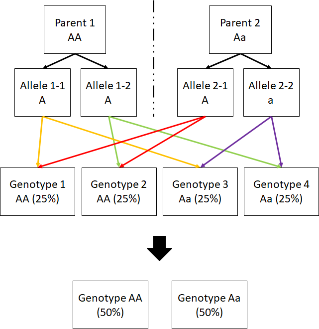 The child genotype probability distribution can be computed by splitting parents’ genotype to alleles and combine them pairwise; alleles from same parent will not be recombined together.
3.1 Constructing New Factors for Decoupled Networks
The factor to compute is \(\phi(Phenotype, Allele_1, Allele_2)\) and approach is similar to 2.2.4; this clue should be sufficient to figure out the rest.
4.2 Constructing Factors with Sigmoid CPDs
It would be clearer if we define the Sigmoid CPD as follows:
Basically, we simply compute the sum of weights of alleles existing in the genotype of interest. You can double check this with the provided example. Hence, once you got this idea, we simply scan through all assigments of genotypes - formed by 4 Gene Copies, then compute \(sigmoid(f(X^1_1, ..., X^1_{n_1}, ..., X^m_{n_m}, Y^1_1, ..., Y^m_{n_m}))\) to fill in the probability distribution.
Week 3: Markov Network Fundamentals
Unlike to week 2 where we have sampleGeneticNetworks.m to test out the implementation, you need to load data structure from .mat files and compare to the instruction.
3.1 Pairwise Factors
You don’t need to do any extra computation for all info are stored in pairwiseModel already and all pairwise factors are defined exactly the same. Notice that pairwiseModel is a matrix whereas .val expected to be a 1-dimensional vector! Once made necesssary change, rebuild the model with
factors = BuildOCRNetwork(allWords, imageModel, pairwiseModel, []);
3.2 Triplet Factors
You need to explicitly build a table of (K*K*K) rows storing factors’ values; its index is corresponding to an assignment of triplet factors, whose factors’ variables are represented in numerical value from \(1\) to \(26\). The tripletList is a factor array with \(2000\) elements, its fields are:
.charstelling you the assignment of top \(2000^{th}\) triplet factors. Assume an assignment is \([x_1, x_2, x_3]\), each such assignment can be converted to table’s index with the formula \(index = x_1 + (x_2-1)*K + (x_3-1)*K^2\); we can derive such formula becausetripletListis essentially a concise representation of our table..factorValtelling you the corresponding value for each assignment in.chars.
Akin to 3.1, you assign the same table to every triplet factor and rebuild the model with
factors = BuildOCRNetwork(allWords, imageModel, pairwiseModel, tripletList]);
3.3 Image Similarity Factors
Compute Similarity Factor
There are (K*K) of character joint assignments in \((C_i, C_j)\) pairs, i.e. \([(1, 1), (1, 2), ..., (26, 26)]\). We will set the similarity score to \(1\) for all but K pairs that having \(C_i = C_j\) to \(ImageSimilarity(I_i, I_j)\).
Compute All Similarity Factor
Readers can figure out how factors is constructed and organized based on nFactors. Once all required steps are made, you can rebuild the model. It takes 5 minutes plus per run.
imageModel.ignoreSimilarity = false;
factors = BuildOCRNetwork(allWords, imageModel, pairwiseModel, tripletList]);
Week 4: Decision Theory
I have faced road block in this last PA - all the local tests are passed but failed after submitting it online, hence I cannot proceed further. The guideline below reflects my understanding and could be wrong since I don’t have actual result validating it. You can check out this useful guideline as well.
Variable Elimination is a useful technique that was not fully explained in the PA, yet your life would be way easier knowing it. In short, this is a Factor Marginalization. Given a factor \(\phi(D)\) having its variable set \(D = X \cup Y\), \(X=\{X_1, X_2, ..., X_m\}\) and \(Y=\{Y_1, Y_2, ..., Y_n\}\). If we want to reduce set of variables of \(\phi\) from \(D\) to \(Y\), it could be performed as follows:
There are 2 observations derived from this:
- \(\mid D \mid \geq 2\): the original variable set \(D\) must have at least \(2\) elements.
- \(\mid Y \mid \geq 1\): the variable set after the reduction must not be an empty set.
The equivalence of \(X\) in VariableElimination is Z.
Note: Makes no assumption about \(Parent(D)\) and \(Parent(O)\), it could be from any \(X_i \in X\). Check out
TestCases.m!
4. Calculating Expected Utility Given A Decision Rule
The instruction is actually clear, but you need to find the correct piece to complete the puzzle. Let’s reformulate it first:
Given a Bayesian network \(I\) with variable set \(X = \{X_1, X_2,... X_n\}\), a decision node \(D\) whose \(Parent(D) = T \subseteq X\), an outcome node \(O \subset X\), an utility node \(U\) whose \(Parent(U) = O \cup D\), let’s compute
We already have \(U(A)\), so the missing factor is \(\phi(A)\), which is in fact \(\phi(Parent(U)) = \phi(O \cup D)\). We can compute this single factor by:
- Apply Factor Product on provided \(\phi(X_i, Parent(X_i)), i \in \mathbb{Z}: i \in [1;n]\) and \(\phi(D, Parent(D))\) to obtain the single factor \(\phi(X, D)\).
- Apply Variable Elimination to obtain \(\phi(Parent(U)) = \phi(O \cup D)\).
- Compute \(\mathop{\mathbb{E}}_I(U)\) by scanning through each assignment of \(Parent(U)\).
6. Maximum Expected Utility With Expected Utility Factors
CalculateExpectedUtilityFactors.m
The new formulation is
and you can follow the same approach in 4.
OptimizeMEU
7.1 Joint Utility Factors
7.2 Linearity of Expectations
The formulation is the same, but implementation is different:
- Compute factor \(O_i = \mathop{\mathbb{E}}_{I'} (d, Parent(d)) , \forall I' \in OutcomeNet(I), \forall O_i \in O\).
- Set \(O_i = VariableElimination(O_i, K_i), K_i = \{\) complementary set between variables of \(O_i\) and decision node \(D \}, \forall O_i \in O\). Now \(O_i\)’s variable set would be \(\{ Parent(U) \cup D \}\).
That’s it, folks! Kudos to any of you made it to this line. It would be great to have your feedback to improve this guideline and help other learners to complete this challenging course 😊.